Week 6: Conjugate Heat Transfer Simulation

Aim:- The aim of this project is to simulate a Conjugate Heat transfer simulation across a pipe. The impacts of 3 grid sizes and supercycling on the results would be examined.

Theory:-

Meaning of Conjugate Heat Transfer

In a heat transfer between a body and fluid flowing past it, the heat transfer inside the body is governed by Fourier's equation wheras the flow in the fluid is governed by the Navier Stokes equation. The solution to such equation gives the temperature and heat flux distributions on the interface. The conjugate heat transfer is used where a solid and a fluid interacts with each other and we need to know the thermal exchange at the interface within the solids and fluids.

There are many conjugate problems in other fields of science. For instance, studying of subsonic-supersonic flows requires conjugation because the subsonic flow is governed by elliptic or parabolic differential equations, while the supersonic flow is governed by hyperbolic differential equation. Every combustion process has two areas containing fresh and burnt gases with different properties . In biology, diffusion processes usually proceed simultaneously in qualitatively different areas (e.g., in membranes) and, therefore, require a conjugation procedure.

Meaning of Supercycling

In super-cycling, the fluid solver is frozen periodically while the heat transfer in the solid is allowed to progress to steady-state. CONVERGE solves the fluid and solid phases in the same simulation without requiring you to stop and restart the simulation. Super-cycling significantly reduces the computational cost of the CHT simulation.

Case Setup

1. Creation of geometry. A concentric pipe with internal diameter of 0.03m and external diameter of 0.04m was created for the purpose of the analysis.
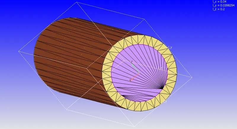
2. After creating the geometry, a diagnosis check was performed in with intersection errors were noticed. These were rectified by selecting the Repair option under Geometry. The Front two faces and the rear faces were selected and deleted.
3. Boundaries were created as listed below
4. 
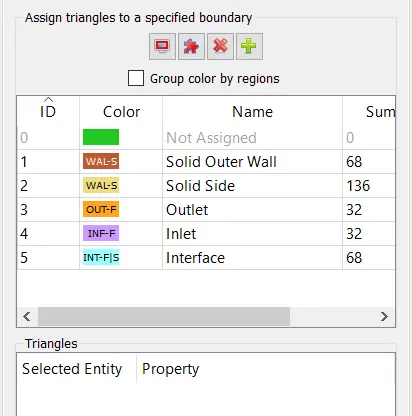
5. The direction of the normals were found to be incorrect and were rectified to ensure the normals are pointing inwards to the direction of fluid flow.
6. After completion of the above steps a diagnosis check was again performed. Non manifold edges were observed and this was as a result of interface between solid and fluid.

Case Setup

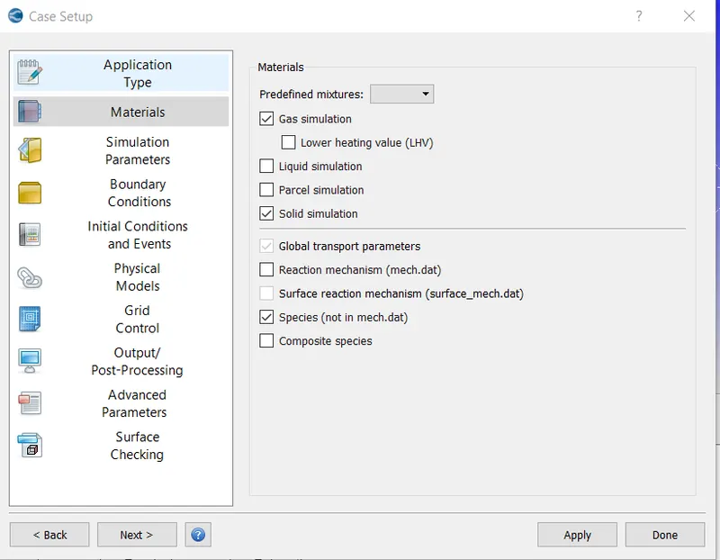
i) Materials:- Gas simulation, Solid Simulation and Species were selected.

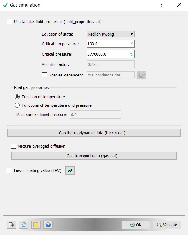
ii) Gas Simulation:- Default retained

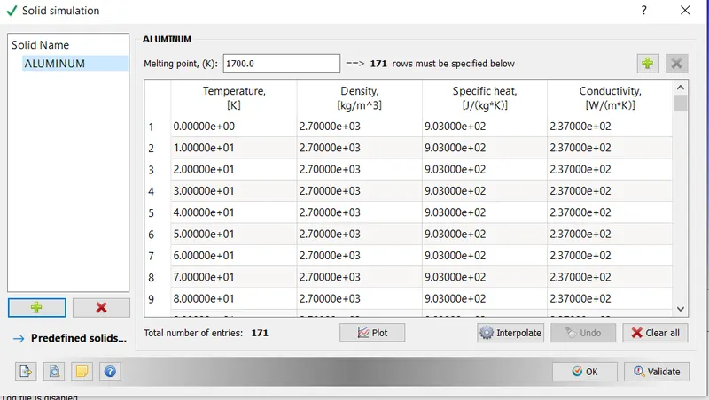
iii) Solid Simulation:- The Material used was Aluminium

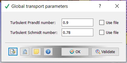
iv) Global Transport Parameters:- Default values retained

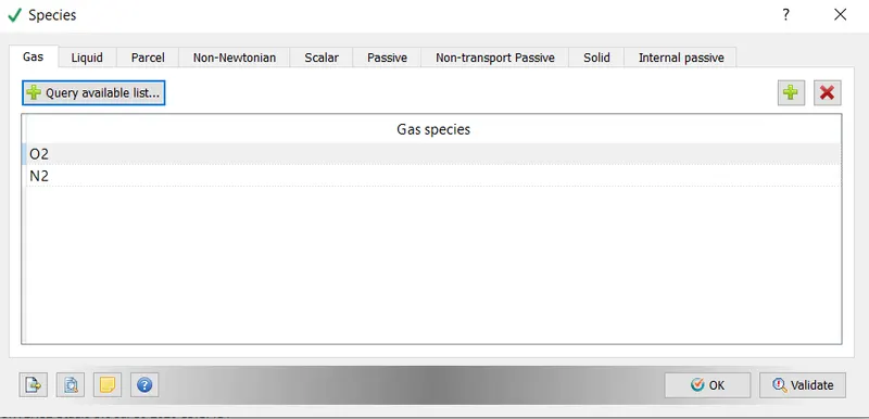
v) Species:-

a) Gas:- O2 and N2

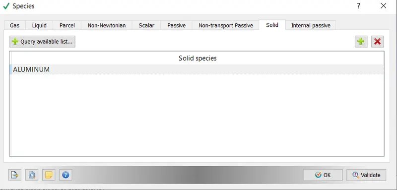
Solid

- Simulation Parameters

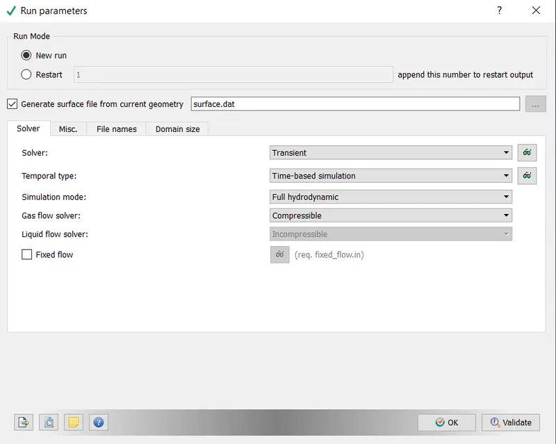
i) Run Parameters:- Simulation set to Transient.

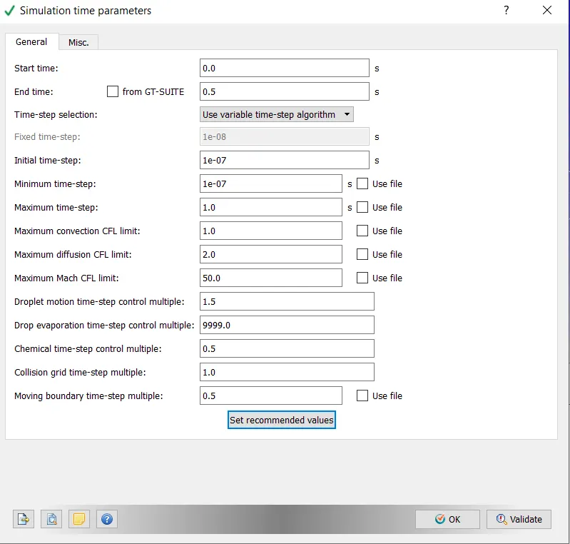
ii) Simulation Time Parameters:- Values set as shown below

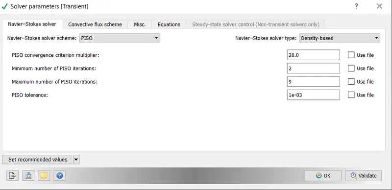
iii) Solver Parameters (Transient):- Defaults value retained

iv) Boundary

- Solid Outer Wall:- A Heat Flux of -10000 W/m^2 is introduced. The negative sign indicates that heat flux is flowing into the pipe.

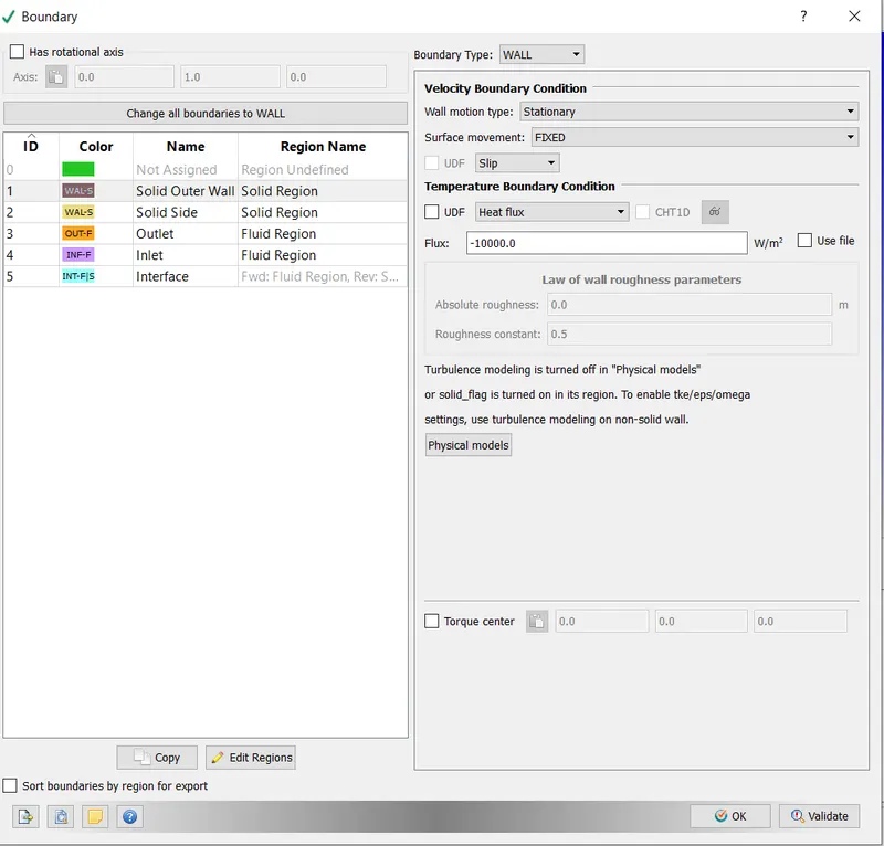
- Solid Side:- Wall motion type is set to stationary, surface movement fixed

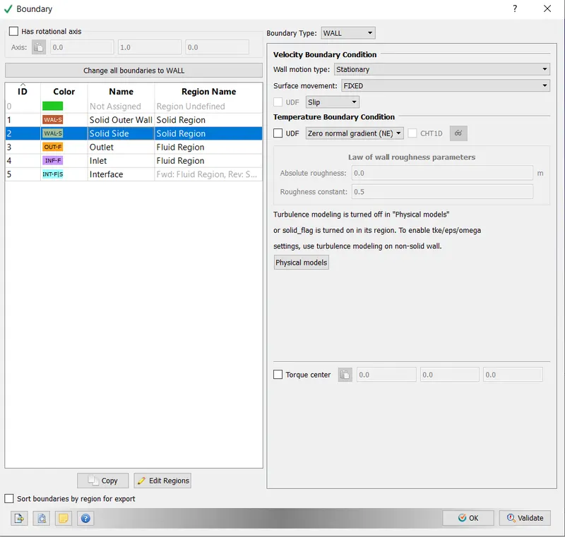
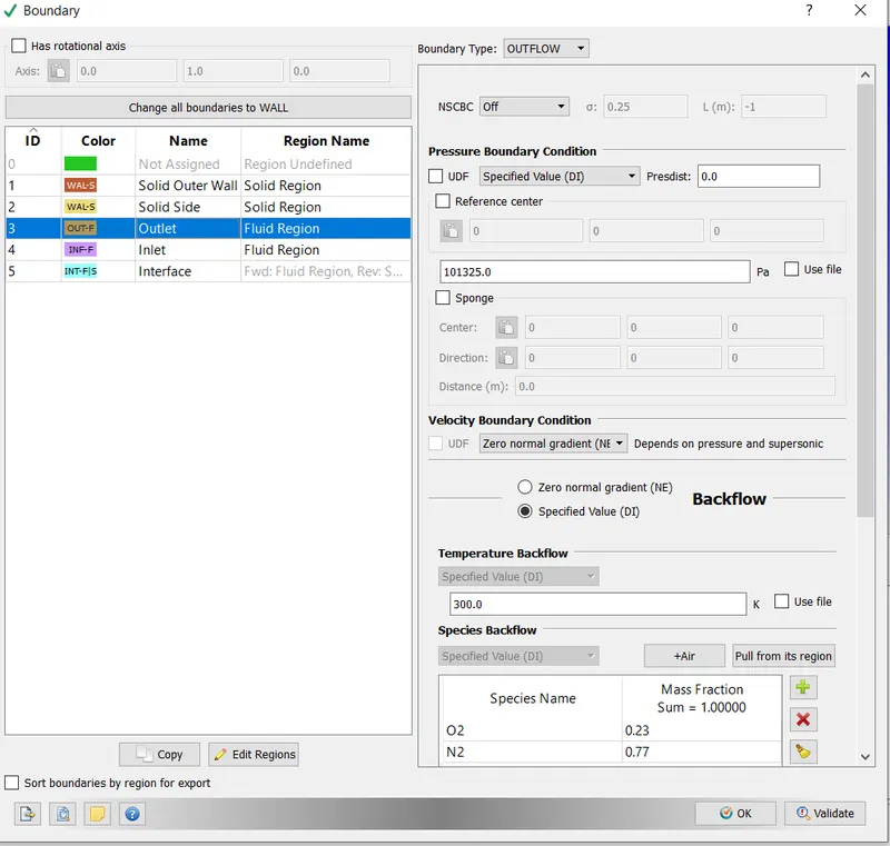
-Outlet:- Pressure Value set to 101325 Pa at the outlet

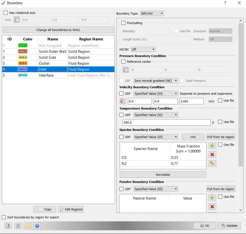
- Inlet:- In the problem it is given that the inlet Reynolds number should be 7000. The value of the inlet velocity is computed from the below formuls

`Re= (rho*u*D)/(mu)`

or

`u=(Re*mu)/(rho*D)`

using the definition (mu/rho) = kinematic viscosity.

The value of Kinematic viscosity at 300 K is 15.69 * 10^-6. Also the diameter is taken to be the internal dia of the pipe which is 0.03m/

Substituitng and solving

`u=(7000*15.69*10^-6)/(0.03)`

u=3.661 m/s

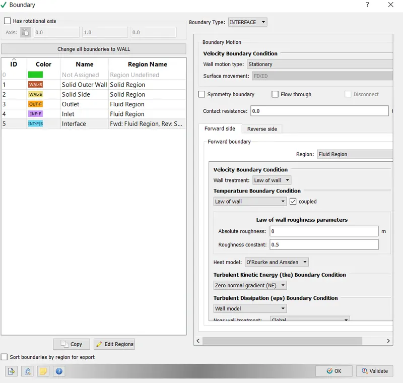
- Interface. The normals on the interface point towards the fluid regionand this is referred to the forward side. The opposite direction which points towards the the solid direction referred to as reverse direction.

Velocity and Temperature boundary condition in forward region set to Law of the Wall

In Reverse region Velocity and temperature set to slip and specified value respectively

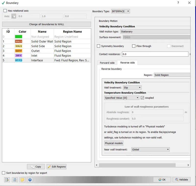
-Regions and Initialization

i) Fluid Region:- Values set as shown below

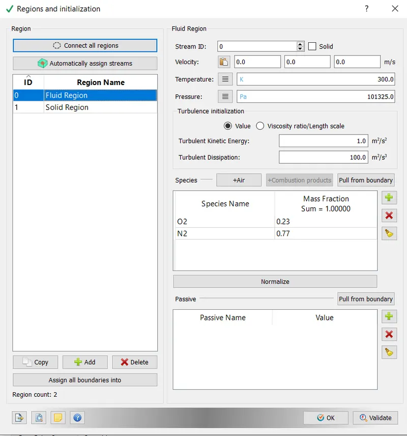
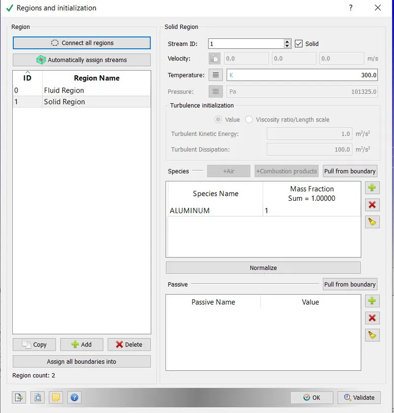
ii) Solid Region:- Stream Id set to 1 and solid box checked

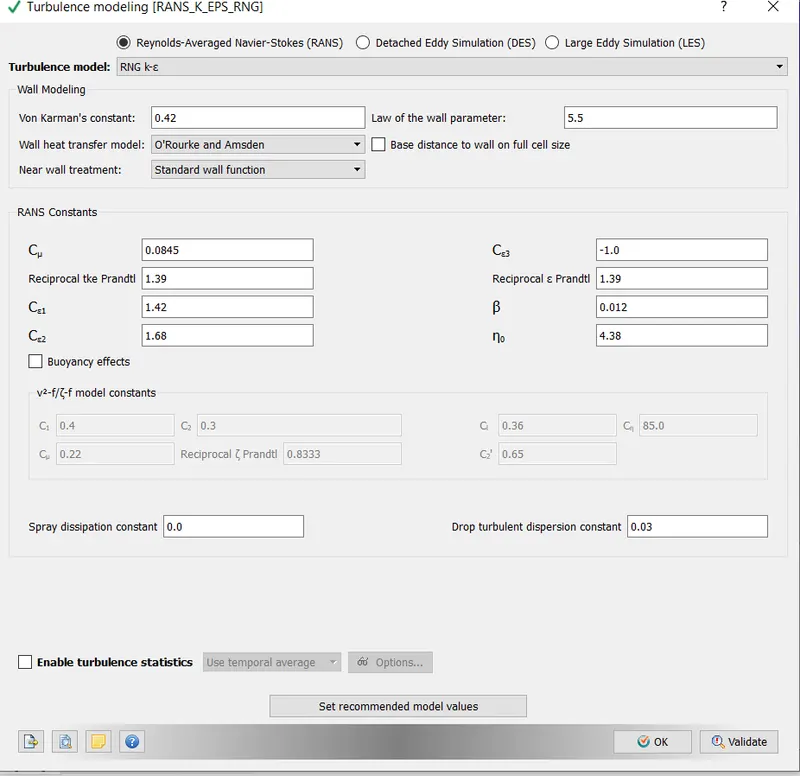
Turbulence Modelling:- k epsilon model is used

-Supercycling was enabled in order to reduce the computational time requried for CHT analysis. A monitor point was created at the outlet. Time length was initially set to 0.05 and then reduced to 0.03,0.02 and 0.01.

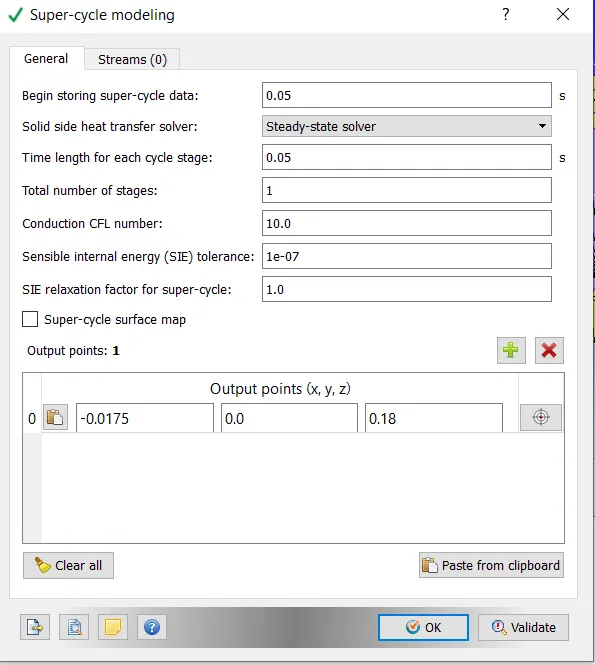
Base grid size was set to 0.004, 0.003,0.0025 and 0.002

In post variable selection, apart from the usual default, wall yplus and heat transfer coefficient was enabled.

The time intervals for writing output files was set as given below

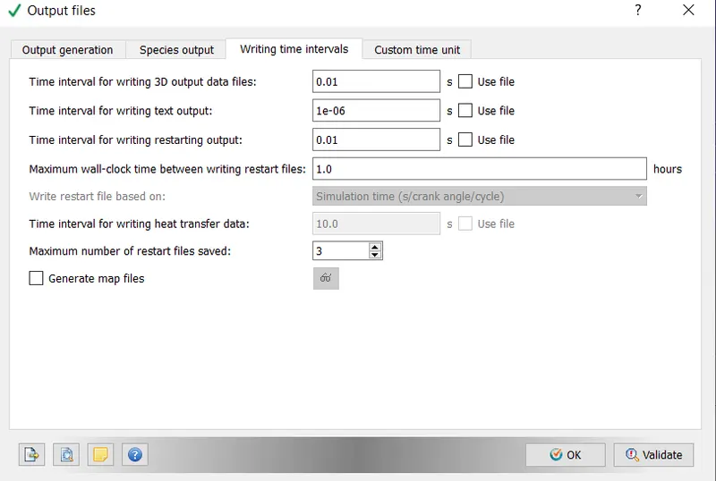
In order to execute the simulation, the directory in which these input files were stored was accessed in Cygwin and the following command was typed "mpiexec.exe -n 4 converge.exe"
After the Simulation was executed, the results were converted into a form which would be compatible with Paraview. This was done using the post_convert.exe command.

Results

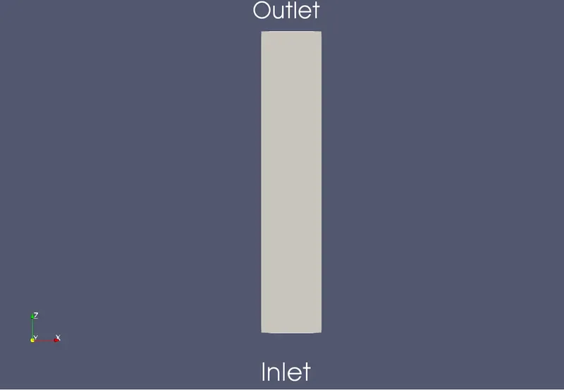
Note, For purposes of the result, the geometry is to be read as shown below

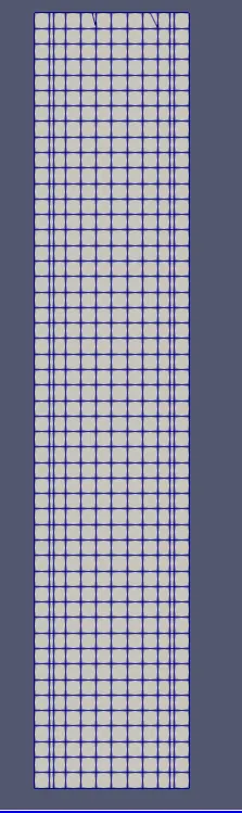
1. Base Mesh. dx=dy=dz= 0.004m . Total number of Cells 5369.

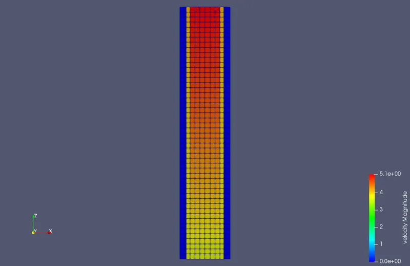
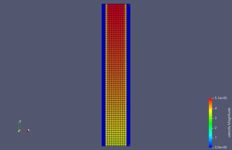
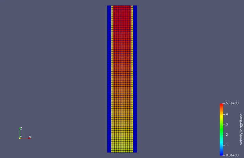
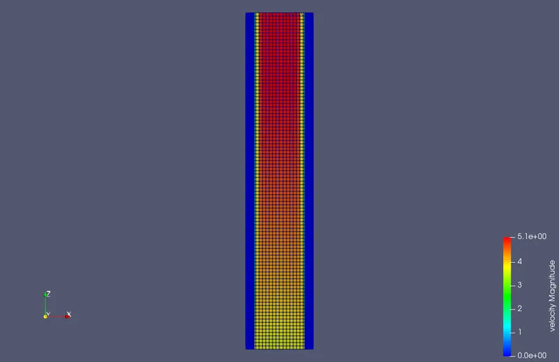
Velocity contour:- From the below plot, the development of velocity profile is observed. At t=0, the velocity at the inlet is 3.661 m/s and outlet is 0m/s. Due to the pressure difference between the inlet and outlet, the flow gradually develops over time. Once the solution converges, we see that a profile develops with velocity 4m/s at the inlet and 5.1 m/s at the outlet. No variation is observed across the solid boundary

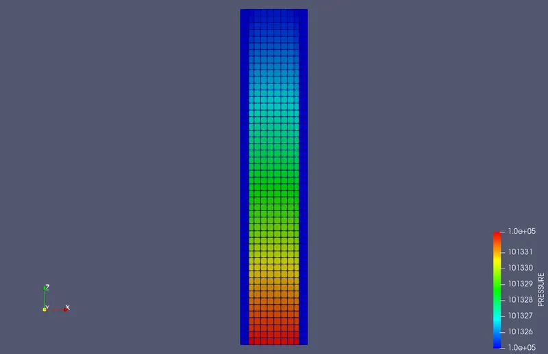
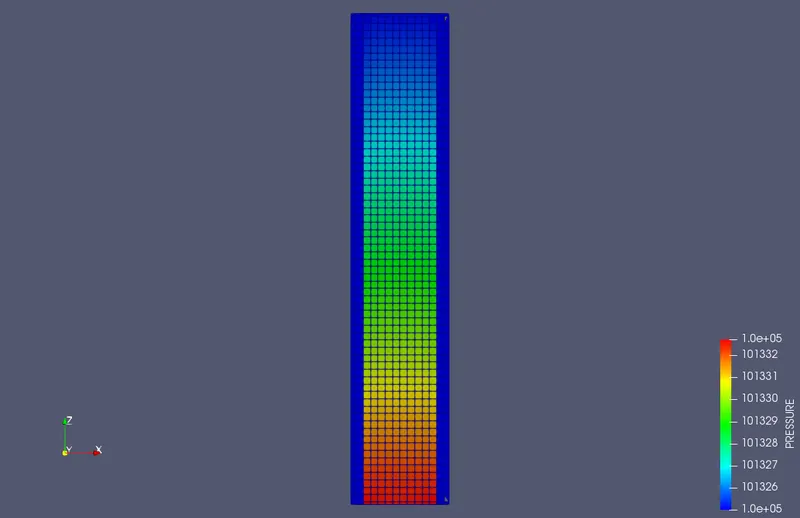
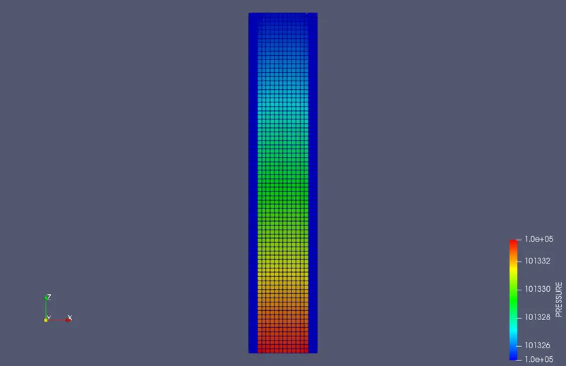
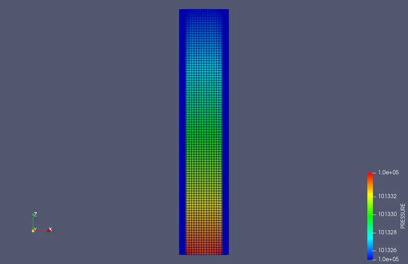
Pressure:- At time 0, a zero normal pressure gradient is set at the inlet and 101325 Pa at the outlet. With the passage of time we note the below profile. The inlet is at a relatively high pressure when compared to the outlet. From the above plot it is noted that inlet ,which is an area of High pressure corresponds to an area of low velocity and outlet, which is an area of low pressure correponds to a high velocity. No variation is observed across solid boundary

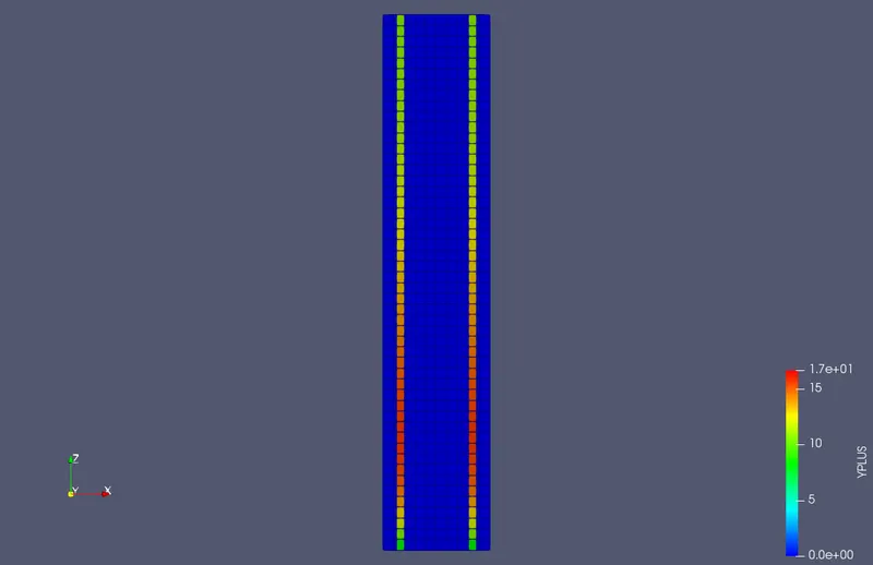
Yplus

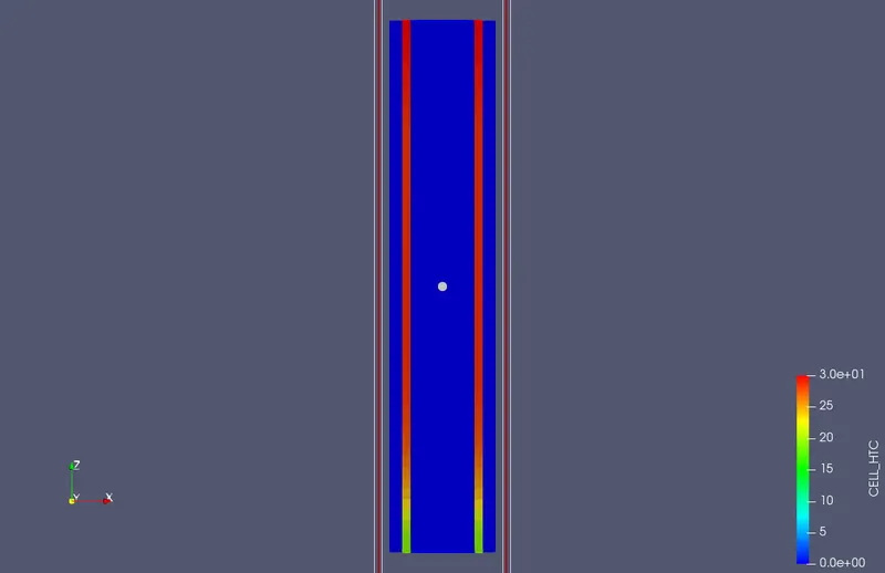
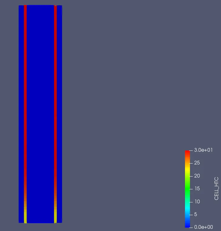
Heat Tranfer Coefficient:- The application of heat flux results in a cell heat transfer coefficient of 30 W/m^2 across the pipe boundary.

Velocity Profile Development:- It is noted that the velocity changes from 0 to a finite value almost instantaneously as the simulation begins

Pressure Profile development:- It is noted that the pressure profile develops almost instantaneouly as the simulation begins

For the 3 refined grids of size 0.003m, 0.0025m and 0.002 m a similar trend was observed as per the base mesh. They are commonly summarized at the end.

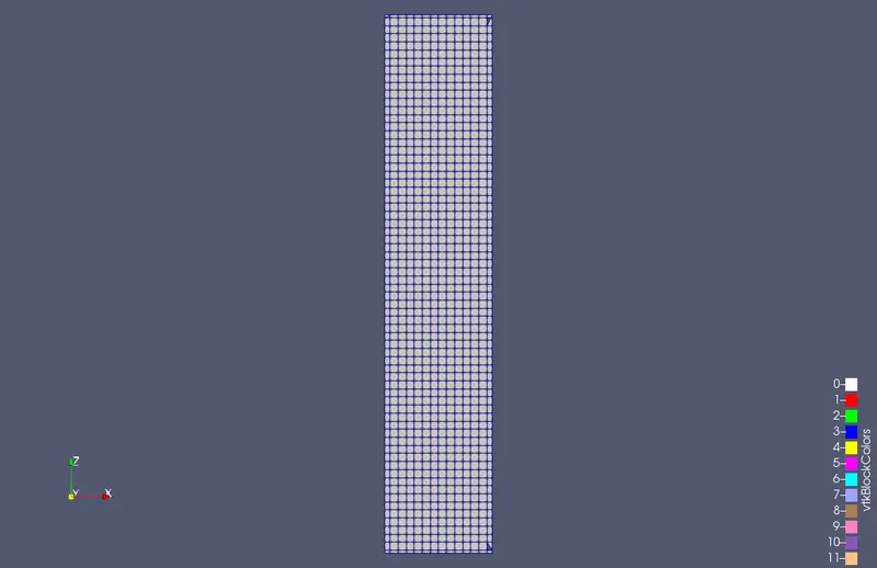
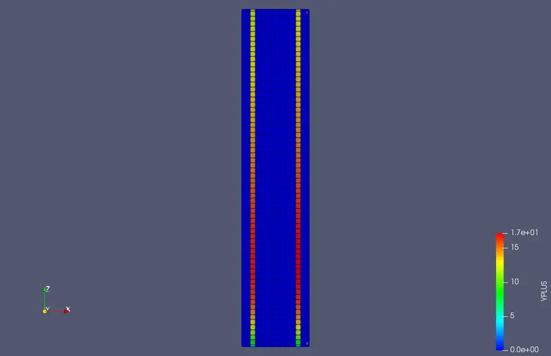
2. Mesh 2, dx=dy=dz=0.003m, Total Cells 12727

Velocity

Pressure

yplus

wall HTC

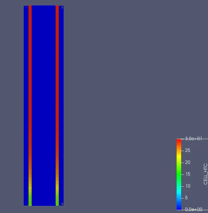
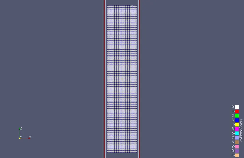
Mesh 3:- dx=dy=dz=0.0025. Total cells 21991

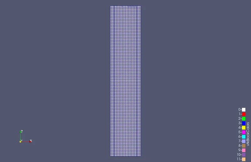
Grid

Velocity

Pressure

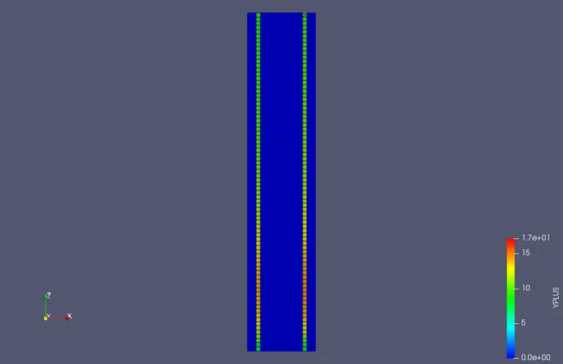
yPlus

Wall HTC

Mesh 4 dx=dy=dz=0.002 Total cells 42951

Velocity

Pressure

Wall HTC

Comparsion between different Meshes

With the refinement of the grid it is seen that gradients in temperature, pressure are observed more clearly. However there is a significant increase in computational time as can be noted in the below table.

Grid Size (m)	Supercycling (time interval)	Time (seconds)
0.004	0.05	378.431
0.003	0.05	861.26
0.0025	0.05	1539.5
0.002	0.05	2134

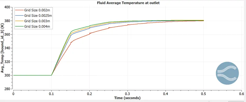
Outlet temperature converging to a particular value:- From the plot below we can see that the outlet temperature converges to the value of about 380 K.

Effect of Supercycling

By reducing the the Supercycling time interval from 0.03 to 0.01, we note that computational time decreases

Supercycling	Grid Size	Time (seconds)
0.03	0.004	353.95
0.02	0.004	313.72
0.01	0.004	286.7

Significane of Y Plus

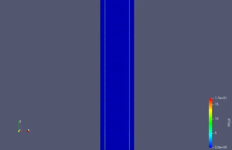
The Y plus values obtained for different grids is given below. With the refinement of grid we note that y plus value decreases.

We need to use wall functions for grids 0.004 and 0.003. For the other two grid sizes the values are below 10 and therefore we are in the viscous sub layer.

Grid Size (m)	y plus
0.004	17
0.003	17
0.0025	10
0.002	5

Other Plots

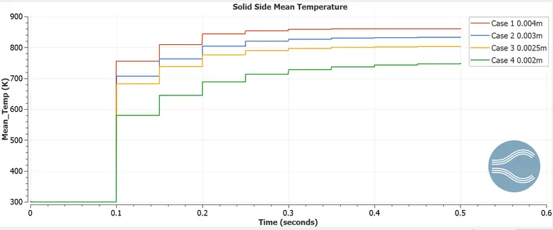
From the above plot we note that there is a variation in the solid side Mean temperature with the refinement of grid. It varies between 830 K for grid with 0.004m and 700K for grid with 0.002 m.

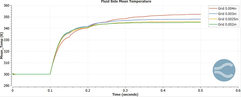
The Fluid Side Mean Temperature is shown above, The variance is much lesser when compared to the solid Mean temperature. For 0.004m it is 355 K and for 0.002m it is about 342K.

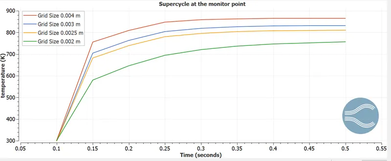
The temperature at the monitor point is shown above for various intervals of supercycling. The value varies from 850K for a coarse grid to 0.002m for a fine grid.

Conclusion:-

From the above analysis we note that

i) Refinement of grid results in clearer plots however at the expense of computational time

ii) Decreasing the SUpercycling time interval results in reduction of computational time

iii)Irrespective of grid size, fluid values converge to a particular value.(380 K)