Week 6 - Multivariate Newton Rhapson Solver

Aim: The aim of this project is to solve the system of coupled ODE's using Multivariate Newton Raphspn Method.

The system of equations which are to be solved are

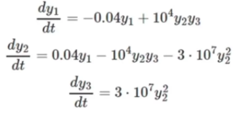
Theory: Combustion calculations often involve a system of coupled ODE. Often these equations cannot by solved analytically and therefore it is required to adopt numerical integral techniques such as Newton Raphsons Method. There are two types of Newton Raphsons techniques, the univariate method for a single variable and Multivariate method for multiple variables. Both these formulations are given below In this project we will be using Multivariate formulation.

Univariate

`y_("new")=y_(guess) -alpha((f(y_(guess))/(fprime(y_(guess)))))`

Multivariate

`y_("new")= y_(guess)-alpha(J^-1)F`

Numerical Procedure for Multivariate Method:

1. Time Differential terms are discretized using the Backward Difference scheme

`(y_1^n - y_1^(n-1))/(Deltat) = -0.04y_1^n + 10^4y_2^ny_3^n`

`(y_2^n - y_2^(n-1))/(Deltat) = 0.04y_1^n -10^4y_2^ny_3^n-3*10^7(y_2^n)^2`

`(y_3^n - y_3^(n-1))/(Deltat) = 3*10^7(y_2^n)^2`

where n and n-1 denote the time steps

2. The components of f vector are defined as below

`f_1^n=y_1^(n-1)-dt(0.04*y_1^n-10^4y_2^ny_3^n)-y_1^n=0`

`f_2^n=y_2^(n-1)-dt(0.04*y_1^n-10^4y_2^ny_3^n-3*10^7(y_2^n)^2)-y_1^n=0`

`f_3^n=y_3^(n-1)+dt(3*10^7(y_2^n)^2)-y_3^n=0`

3. Jacobian Matrix is defined as

`J=[[(delf_1^n)/(dely_1^n),(delf_1^n)/(dely_2^n),(delf_1^n)/(dely_3^n)],[(delf_2^n)/(dely_1^n),(delf_2^n)/(dely_2^n),(delf_2^n)/(dely_3^n)],[(delf_3^n)/(dely_1^n),(delf_3^n)/(dely_2^n),(delf_3^n)/(dely_3^n)]]`

4. Differential terms of Jacobian matrix are calculated as

`(delf_i)/(dely_i) =( f_i(y_i+Deltay_i)-f_i(y_i))/(Deltay_i)`

Coding Procedure:

1. Outer Time Integration loop
2. Assembling ODE system
3. Newton Raphson run till convergence
4. Get new Values and perform updates
5. End Time loop

Code

"""
Current example ODEs:
    d(y1)/dt = -0.04*y1 +(10^4)*y2*y3
    d(y2)/dt = 0.04*y1-10^4y2*y3-3*10^7*y_2^2
    d(y3)/dt= 3*(10^7)*(y2)^2
"""
import matplotlib.pyplot as plt
import numpy as np
from numpy.linalg import inv

# Function to find components of F matrix, roots of ODE
def f1(y1o,y1n,y2n,y3n,dt):
    return y1o-0.04*dt*y1n+1e4*dt*y2n*y3n-y1n
def f2(y2o,y1n,y2n,y3n,dt):
    return y2o+0.04*dt*y1n-1e4*dt*y2n*y3n-3e7*dt*(pow(y2n,2))-y2n
def f3(y3o,y1n,y2n,y3n,dt):
    return y3o + 3e7*dt*pow(y2n,2) -y3n

#Jacobian Matrix
def jacob(ny,oy,dt):
    dy=1e-5
    J=np.zeros((3,3))
    J[0,0]=(f1(oy[0],ny[0]+dy,ny[1],ny[2],dt)-f1(oy[0],ny[0],ny[1],ny[2],dt))/dy
    J[0,1]=(f1(oy[0],ny[0],ny[1]+dy,ny[2],dt)-f1(oy[0],ny[0],ny[1],ny[2],dt))/dy
    J[0,2]=(f1(oy[0],ny[0],ny[1],ny[2]+dy,dt)-f1(oy[0],ny[0],ny[1],ny[2],dt))/dy
    
    J[1,0]=(f2(oy[1],ny[0]+dy,ny[1],ny[2],dt)-f2(oy[1],ny[0],ny[1],ny[2],dt))/dy
    J[1,1]=(f2(oy[1],ny[0],ny[1]+dy,ny[2],dt)-f2(oy[1],ny[0],ny[1],ny[2],dt))/dy
    J[1,2]=(f2(oy[1],ny[0],ny[1],ny[2]+dy,dt)-f2(oy[1],ny[0],ny[1],ny[2],dt))/dy
    
    J[2,0]=(f3(oy[2],ny[0]+dy,ny[1],ny[2],dt)-f3(oy[2],ny[0],ny[1],ny[2],dt))/dy
    J[2,1]=(f3(oy[2],ny[0],ny[1]+dy,ny[2],dt)-f3(oy[2],ny[0],ny[1],ny[2],dt))/dy
    J[2,2]=(f3(oy[2],ny[0],ny[1],ny[2]+dy,dt)-f3(oy[2],ny[0],ny[1],ny[2],dt))/dy
    
    return J

#Time array

tstart=0
tstop=600
dt=2
n=(tstop-tstart)/dt +1
t= np.linspace(tstart,tstop,int(n))

oy=np.zeros((3,1))
oy[0]=1
F=np.copy(oy)
ny=np.zeros((3,1))

err=9e9
alpha=1
tol=1e7
count=1
y1=[1]*len(t)
y2=[0]*len(t)
y3=[0]*len(t)

# Newton Raphson iteration

for i in range(1,len(t)):
    y1o=oy[0]
    y2o=oy[1]
    y3o=oy[2]
    gy=np.copy(oy)
    
    while err>=tol:
        jac=jacob(ny,oy,dt)
        F[0]=f1(y1o,gy[0],gy[1],gy[2],dt)
        F[1]=f2(y2o,gy[0],gy[1],gy[2],dt)
        F[2]=f3(y3o,gy[0],gy[1],gy[2],dt)
        ny=gy-alpha*np.matmul(inv(jac),F)
        err=max(abs(ny-gy))
        gy=ny
        count+=1
    oy=ny
    y1[i]=ny[0]
    y2[i]=ny[1]
    y3[i]=ny[2]
    
    logmessage='Time={0} sec,iterations={1},y1={2},y2={3},y3={4}'.format(round(t[i],5),count,ny[0],ny[1],ny[2])
    print(logmessage)
    count=0
    err=9e9
plt.plot(t,y1,label='$y1$')
plt.plot(t,y2,label='$y2$')
plt.plot(t,y3,label='$y3$')
plt.xlabel('Time(sec)')
plt.ylabel('$yi$')
plt.title('Multivariate Newton Raphson Solution for dt='+str(dt)+' sec')
plt.legend()
plt.grid(True)
plt.show()

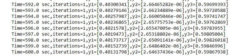
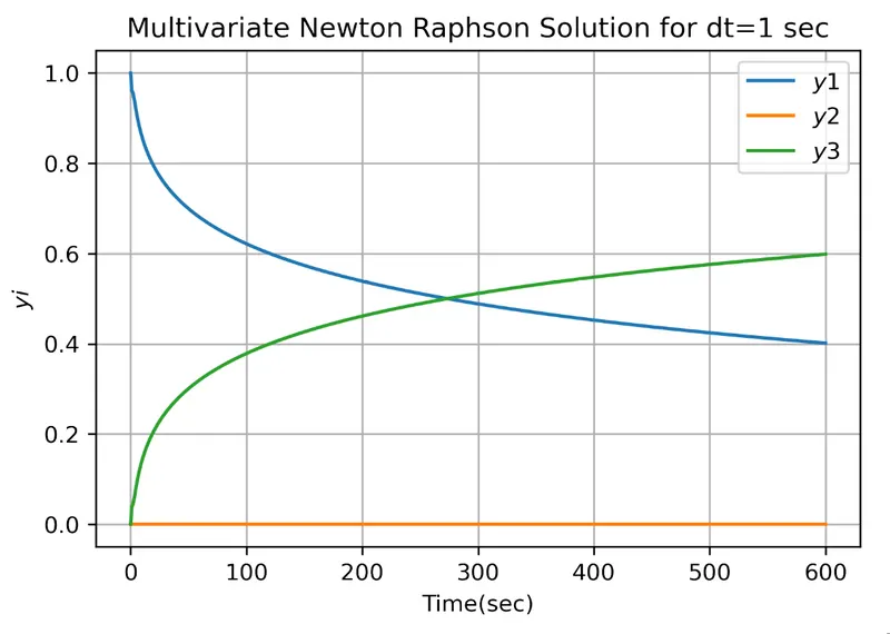
At dt=1 sec

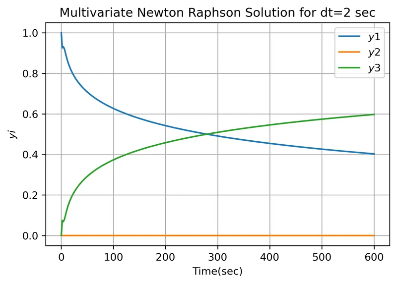
At dt=2

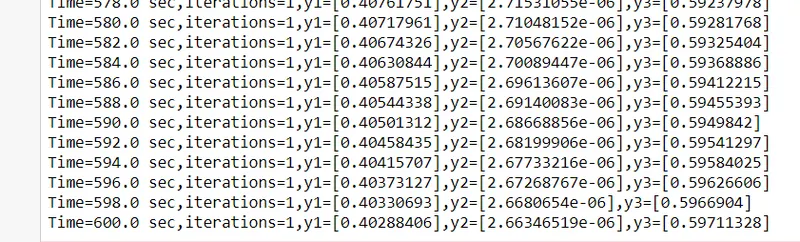
At dt=0.2

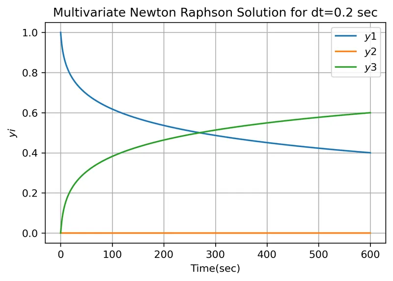
In the implicit formulation, all timesteps approximately give the same values. The ideal time step depends on order of accuracy desired. The system of ODE can be solved for a range of time steps to and the difference in values can be computed to determine the order of accuracy.

Conclusion:

In this project, solving the coupled ODE using Multivariate Newton Raphson integration technique has been understood.