Week 7: Shock tube simulation project

Aim:- The aim of the project is to simulate the flow across a shock tube. We intend to study the pressure and temperature distribution over time. Also we intend to study the variation of cell count over time.

Theory:-

The shock tube is an instrument used to replicate and direct blast waves at a sensor or a model in order to simulate actual explosions and their effects, usually on a smaller scale. Shock tubes (and related impulse facilities such as shock tunnels, expansion tubes, and expansion tunnels) can also be used to study aerodynamic flow under a wide range of temperatures and pressures that are difficult to obtain in other types of testing facilities. Shock tubes are also used to investigate compressible flow phenomena and gas phase combustion reactions. More recently, shock tubes have been used in biomedical research to study how biological specimens are affected by blast waves

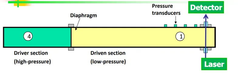
Basic Concept

1. High pressure driver gas expands upon diaphragm opening, creating shock wave
2. Test gas is instantaneously compressed and heated to combustion temperatures
   by incident and reflected shocks.
3. High-temperature experiments monitored near endwall

Shock Tube Characteristics

1. Instantaneous heating/compression from shock waves
2. Accurately known incident- and reflected-shock conditions (from incident shock MS)
3. Wide range of post-reflected shock Temperature and Pressure (600-4000 K, 0.1-1000 atm)

Case Setup

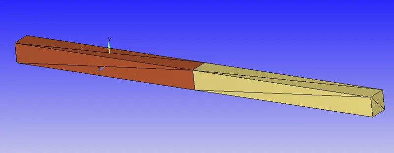
1. Geometry:- STL file is imported into Converge. The geometry for consideration is given below

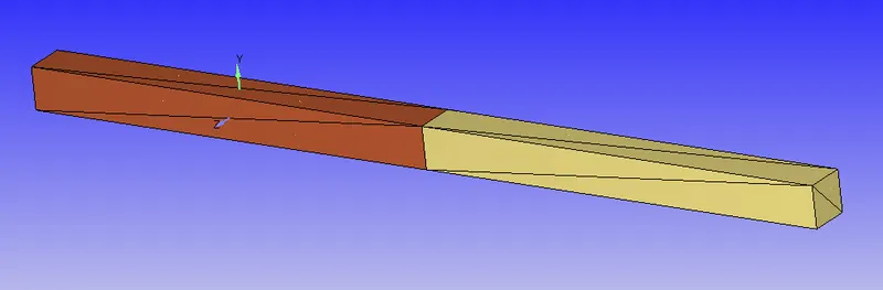
It consists of a tube which separated into two regions of different pressure. Nitrogen(dark brown) occupies a High pressure region wheras oxygen occupies the low pressure region (light brown).

2. Diagnosis:- Upon running a diagnosis check, it was noted that there were a number of Non manifold edge problems.

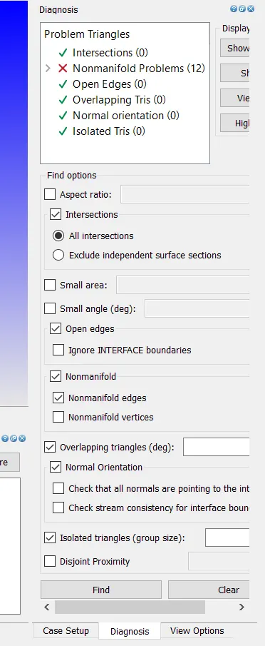
This was due to the presence of a diaphragm inside the tube. This was deleted for the purpose of this analysis. With the deletion, the problem of non manifold edges disappeared.

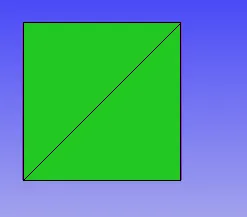
3. Transform Normal:- The normals of the geometry were pointing outwards. This was transformed to ensure the normals pointed inwards.

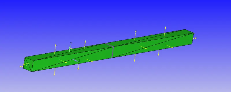
Normals pointing inwards

4. Case Setup

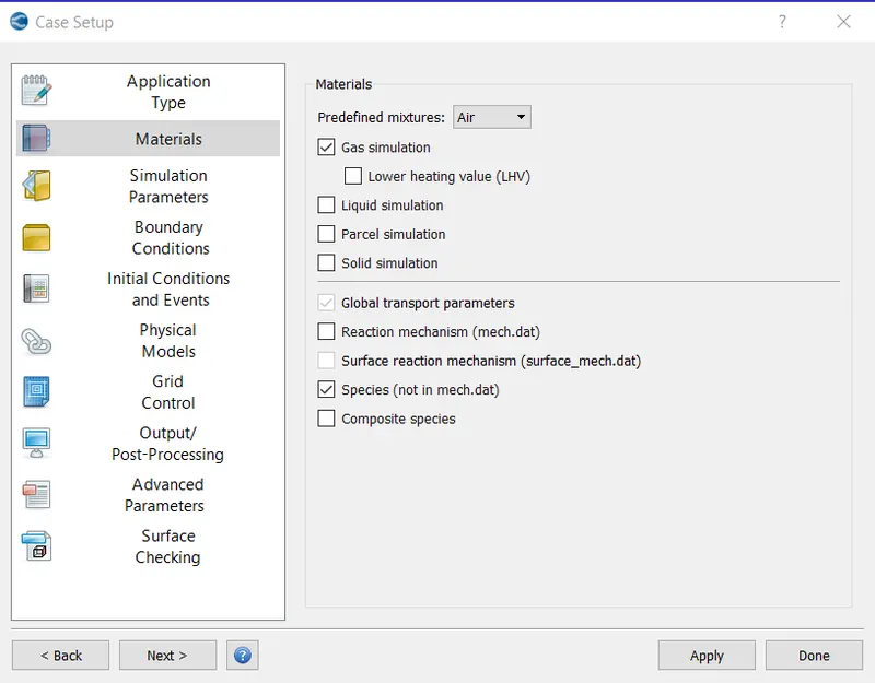
a) Materials:- Pre defined mixture was set to Air, Gas and species selected

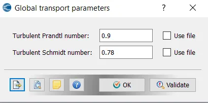
b) Global Transport Properties:- Default values retained

c) Species:- O2 and N2 entered.

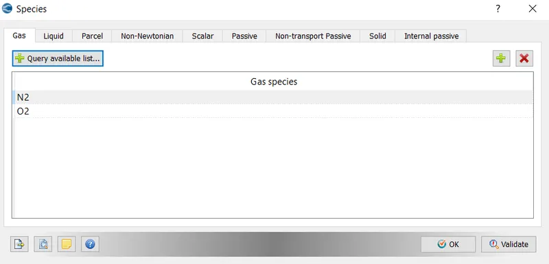
d) Simulation Parameters:-

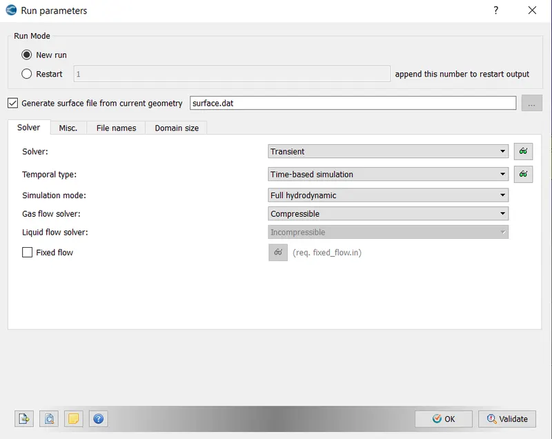
i) Run Parameters:- Transient enabled

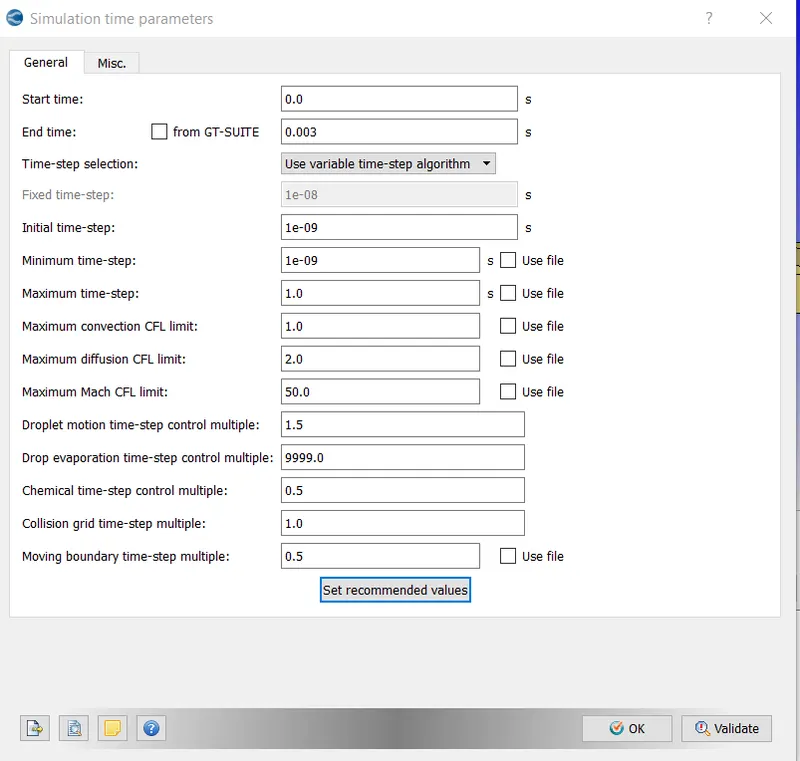
ii) Simulation Time Parameters:- Values set as shown below.

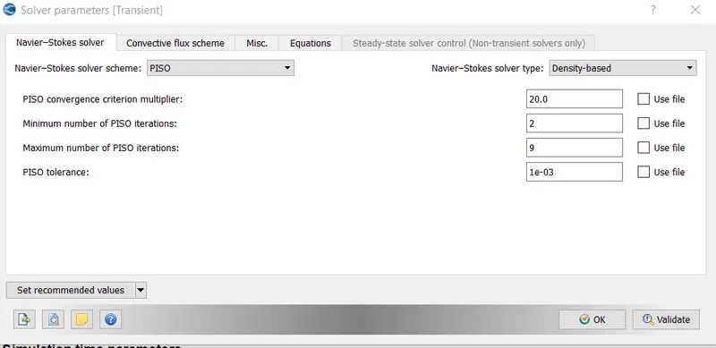
iii) Solver Parameters :- Solver scheme set to PISO

Regions and Initialization

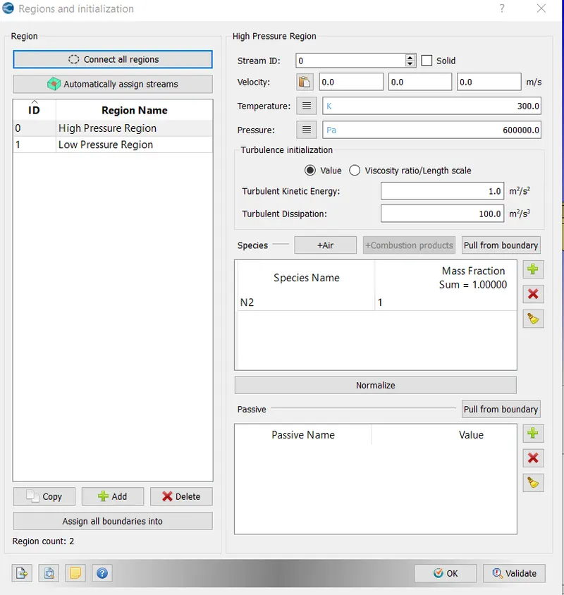
- High Pressure Region:- Pressure set to 6 bar. Mass fraction of N2 set to 1.

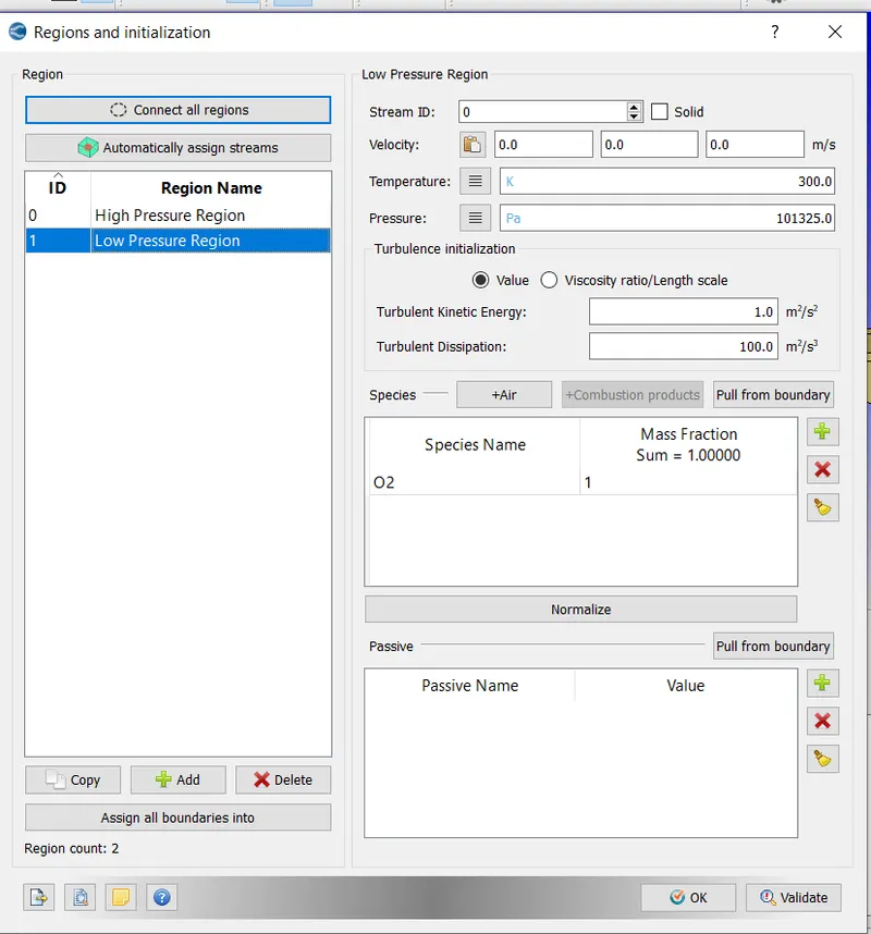
-Low Pressure Region- Pressure set to atm, Mass fraction of O2 is 1.

- Events: Events are used when two boundaries are in contact with each other and there is no boundary between them. the event flag creates traingles in between two regions called disconnect triangles

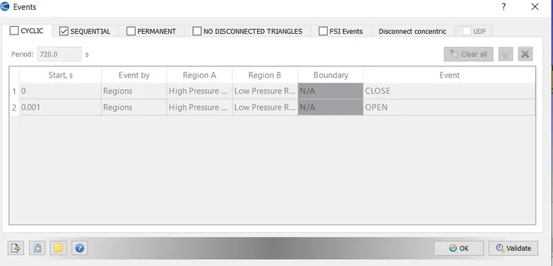
Events can be cyclic, sequential or permanent. Traingles are crated when there is supposed to be no interaction between two regions and disconnected when there is suppossed to be an interaction.

Boundary

High Pressure region. Wall motion type set to Stationary. Surface movement set to fixed.

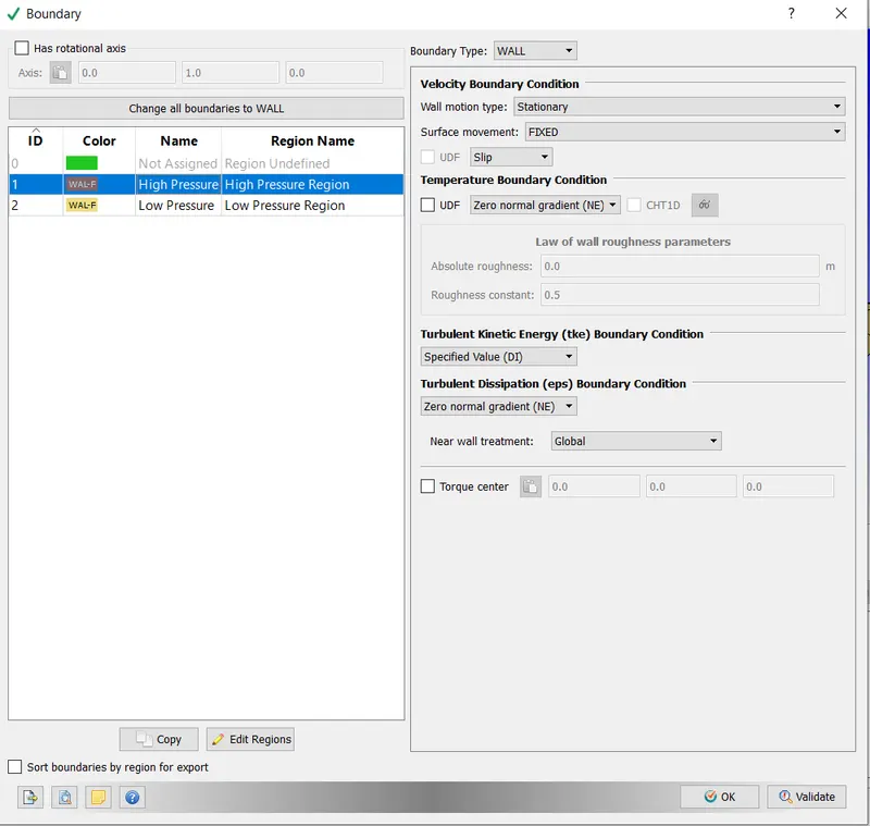
Low Pressure Region: Wall motion type set to Stationary. Surface movement set to fixed.

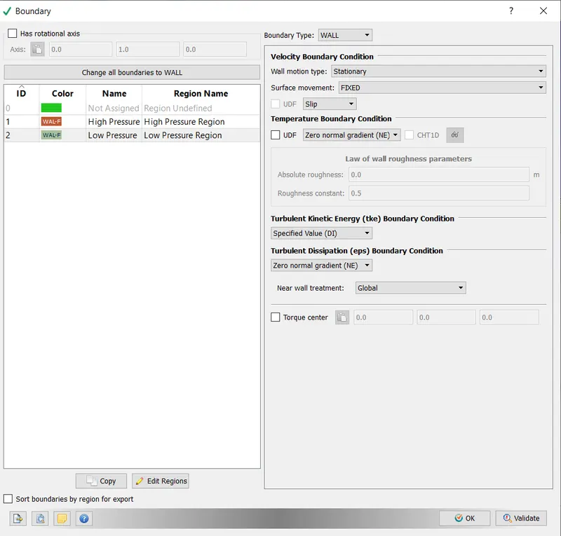
also the Group colour by region is enabled.

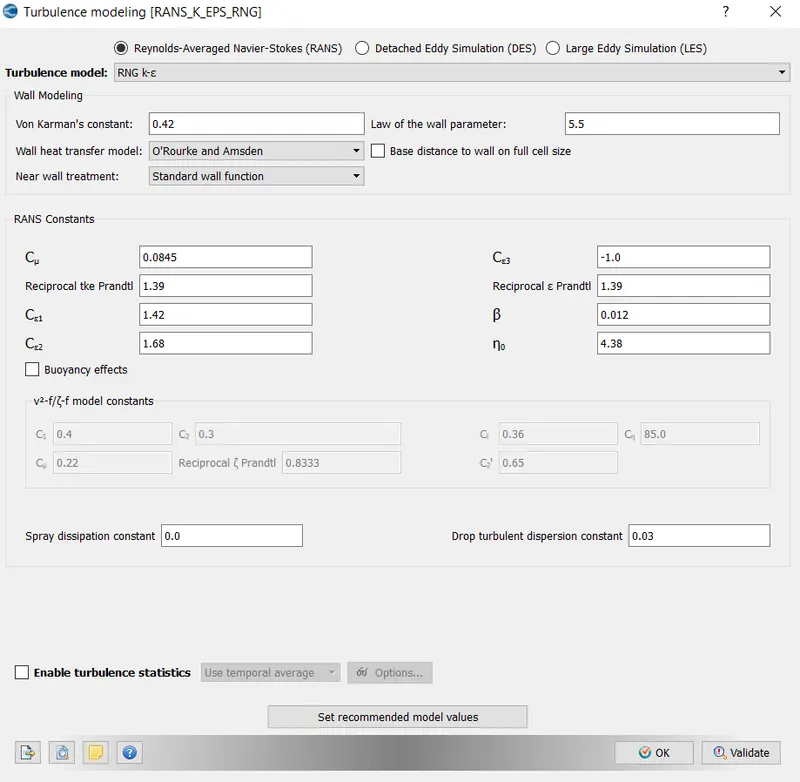
- Physical Models:- Turbulence modelling set to RNG K epsilon

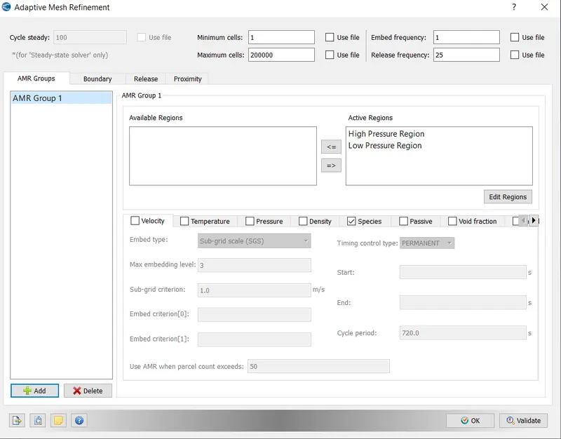
-Adaptive Mesh Refinement:- Adaptive mesh refinement feature in Converge was enabled. This was done to increase mesh resolution in the vicinity of the boundary such that cell size is sufficient to predict the boundary layer effects.

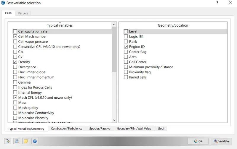
- Post Variable selection

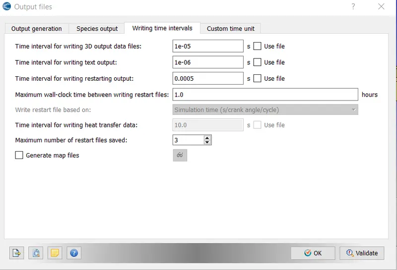
Output files writing time interval is set as shown below

In order to execute the simulation, the directory in which these input files were stored was accessed in Cygwin and the following command was typed "mpiexec.exe -n 4 converge.exe"
After the Simulation was executed, the results were converted into a form which would be compatible with Paraview. This was done using the post_convert.exe command.

Results

1) Base Mesh:- Mesh with dx=dy=dz=1mm is shown below.

Mesh with AMR:- Mesh with Adaptive Mesh refinement is shown below. Converge monitors the curvature properties and whenever it is more than the defined SGS criterion, it will refine the mesh

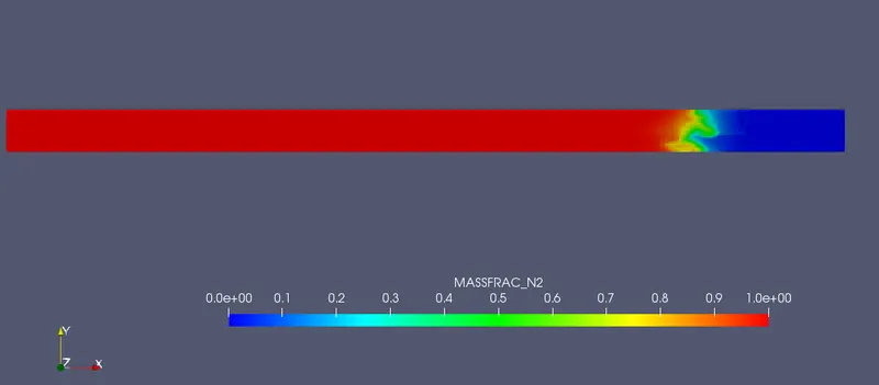
2) Mass Fraction of N2 contour:- In the below animation we observe that N2 which occupies a high pressure region pushes O2 from the low pressure region when the diaphragm breaks. Also the O2 region reflects and pushes it back to the N2 region This back and forth motion continues and eventually it reaches converges to a steady state.

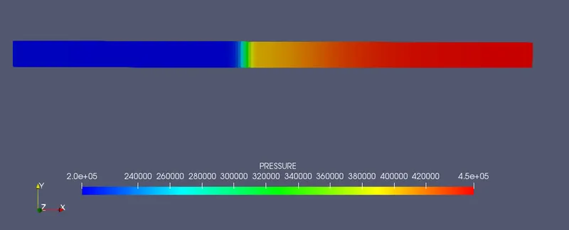
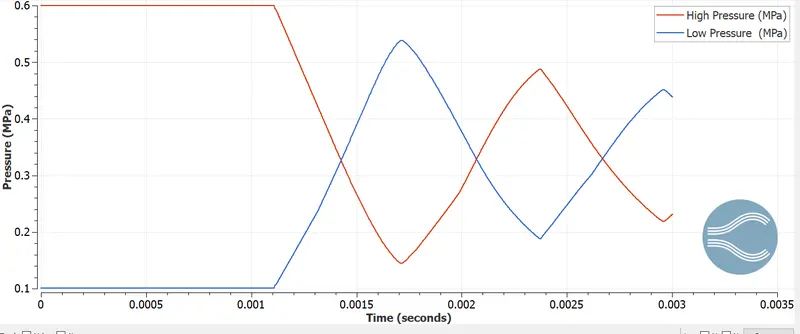
3) Pressure Contour:- A shock wave is generated once the diaphragm is ruptured.Creation of shock wave is characterised by abrupt decrease in pressure on the high pressure side initially . The reflected waves generate a back pressure resulting in an increase in pressure on the low pressure side, which then moves on to cover the high pressure side. THere is an alternate fluctuation in pressure between regions as can be observed from the below animation as well as the plot

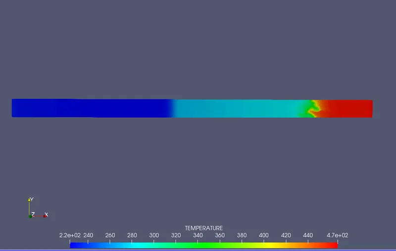
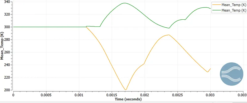
4) Temperature Contour:- The temperature contour also follows the same pattern as pressure. Temperature initially decreases in N2 region initially. Reflected waves generate a backpressure causing increasing in temperature on the O2 side which then covers the high pressure side. Alternate fluctuation in Temperature can be observed in the animation as well as the line plot

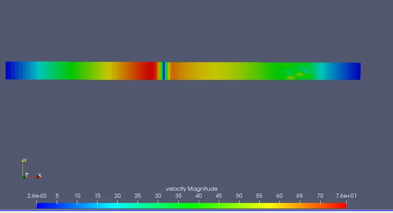
Velocity:- A similar velocity profile characterised by fluctuations similar to pressure and temperature can be seen from the animation below.

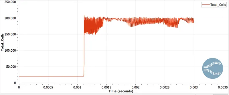
Cell Count:- The plot below shows the variation of mesh size as a function of time. At 0.001sec when the diaphragm gets destroyed, the event is characterized by destruction of disconnected cells. Therefore a sudden spike with rapid fluctuations is observed. Further variation post t=0.001sec can be explained due to interaction of high and low pressure regions during which AMR gets activated.

Conclusion:

In the above analysis, flow through shock wave is simulated,

Bursting of the diaphragm results in creation of shock waves. Compression waves propogate in the the low pressure section wheras expansion waves in the high pressure section. Shock waves get refracted back resulting in mixing of fluid.

The mixing is characterised by abrupt fluctuation in pressure, density and velocity as can be observed from the plots.

Cell count varies once the shock wave is created. The variation is primarily due adptive mesh refinement and rupturing of diaphragm.