Week 3 - Taylor table method and Matlab code
Fourth Order Approximation of Second order derivative
1) Central Difference Scheme:-
`(del^2f)/(delx^2)~=f''(x) +Deltax^4f^6(x)(CONSTANT)=((a.f(i-2)+b.f(i-1)+c.f(i)+d.f(i+1)+e.f(i+2))/(Deltax^2))`
Using Taylors table Method we expand each of the terms about f(i)
`f(i-2)=f(i)-2*Deltax*f'(i) +((2*Deltax)^2/(2!)).f''(i)-((2*Deltax)^3/(3!))*f'''(i)+((2.Deltax)^4/(4!)).f''''(i)+((2.Deltax)^5/(5!)).f'''''(i)`
Similarly other terms such as f(i-1),f(i), f(i+1) and f(i+2) are expanded about f(i). This gives a system of equation with 5 equation and 5 unknowns.
We then form a matrix equation of the form AX=B. A matrix consists of coefficients of 1st,second, third,fourth and fifth order dervatives. Since second order is of concern to us , we set it equal to 1. Remaining are set to 0.
System of Equations for CDS
b+c+d+e+g=0
-2b-c+e+2g=0
2b+c/2+e/2+2g=1
-(4/3)*b-c/6+e/6+(4/3)*g=0
(16/24)*b +c/24 +e/24+(16/24)*g=0
-A Matrix for central Difference scheme
| f'(i) | f''(i) | f'''(i) | f''''(i) | f'''''(i) |
| 1 | 1 | 1 | 1 | 1 |
| 2 | -1 | 0 | 1 | 2 |
| 2 | 1/2 | 0 | 1/2 | 2 |
| -1 1/3 | 1/6 | 0 | 1/6 | 1 1/3 |
| 16/24 | 0.041666667 | 0 | 0.041667 | 16/24 |
- Skewed Right Handed difference
`(del^2f)/(delx^2)~=a.f(i) +b.f(i+1)+c.f(i+2)+d.f(i+3)+e.f(i+4) +g.f(i+5)`
The system of equations for this scheme is given below
a+b+c+d+e+g=0
b+2c+3d+4e+5g=0
b/2 +2c+(9/2)*d+8e+(25/2)*g=1
b/6 +(8/6)*c +(27/6)*d+(64/6)*e+(125/6)*g=0
b/24+(16/24)*c +81/24)*d+(256/24)*e+(625/24)*g=0
b/20+(32/120)*c +(243/120)*d +(1024/120)*e +(3125/120)*g =0
Taylors table for Skewed RIght handed scheme
| f'(i) | f''(i) | f'''(i) | f''''(i) | f'''''(i) | f''''''(i) |
| 1 | 1 | 1 | 1 | 1 | 1 |
| 0 | 1 | 2 | 3 | 4 | 5 |
| 0 | 1/2 | 2 | 4 1/2 | 8 | 12 1/2 |
| 0 | 1/6 | 1 1/3 | 4 1/2 | 64/6 | 125/6 |
| 0 | 0.04 | 16/24 | 81/24 | 256/24 | 625/24 |
| 0 | 1/120 | 32/120 | 243/120 | 1024/120 | 3125/120 |
Skewed Left Handed scheme
`(del^2f)/(delx^2)~=a.f(i) +b.f(i-1)+c.f(i-2)+d.f(i-3)+e.f(i-4) +g.f(i-5)`
System of equations
a+b+c+d+e+g=0
b+2c+3d+4e+5g=0
b/2 +2c+(9/2)*d+8e+(25/2)*g=1
b/6 +(8/6)*c +(27/6)*d+(64/6)*e+(125/6)*g=0
b/24+(16/24)*c +81/24)*d+(256/24)*e+(625/24)*g=0
b/20+(32/120)*c +(243/120)*d +(1024/120)*e +(3125/120)*g =0
| f'(i) | f''(i) | f'''(i) | f''''(i) | f'''''(i) | f''''''(i) |
| 1 | 1 | 1 | 1 | 1 | 1 |
| 0 | 1 | 2 | 3 | 4 | 5 |
| 0 | 1/2 | 2 | 4 1/2 | 8 | 12 1/2 |
| 0 | 1/6 | 1 1/3 | 4 1/2 | 64/6 | 125/6 |
| 0 | 0.04 | 16/24 | 81/24 | 256/24 | 625/24 |
| 0 | 1/120 | 32/120 | 243/120 | 1024/120 | 3125/120 |
Proof of Order of Accuracy
1) Central Order Difference scheme: Order of accuracy is given by
P=N-Q+1
where P= Order of Accuracy
N= Number of stencil points
Q= Order of derivative under calculation
here N-5, Q =2
P=5-2+1=4
Therefore, CDS scheme is 4th order accurate.
2) Skewed Right and Left schemes:- Order of acccuracy
P=N-Q
P= 6-2=4;
Therefore, Skewed Right and left schemes are 4th order accurate
Matlab code for computation of second order approximation of function f(x)=exp(x)*cos(x)
%Main Program
clear all
close all
clc
x=pi/3;
dx=linspace(pi/10,pi/400,100);
analytical_d=-2*exp(x)*sin(x);
A=[1 1 1 1 1;
  -2 -1 0 1 2;
   2 1/2 0 1/2 2;
   -4/3 -1/6 0 1/6 4/3;
    16/24 1/24 0 1/24 16/24];
B=[0;0;1;0;0];
X= linsolve(A,B);

C=[1 1 1 1 1 1 ;0 1 2 3 4 5;0 1/2 2 9/2 8 25/2;0 1/6 8/6 27/6 64/6 125/6 ;0 1/24 16/24 81/24 256/24 625/24 ; 0 1/120 32/120 243/120 1024/120 3125/120];
D= [0;0;1;0;0;0];
Y=linsolve(C,D);


% E=[1 1 1 1 1;4 3 2 1 0; 16 9 4 1 0; 64 27 8 1 0; 256 81 16 1 0]
% F= [0;0;2;0;0]
% Y=linsolve(E,F)
x=pi/3;
for i=1:length(dx)
    [c_d,sr_d,sl_d]=secondorder(x,dx(i),X,Y);

    Central_diff(i)=c_d;
    Error_cd(i)= abs(Central_diff(i)-analytical_d);
    Skewedr_diff(i)=sr_d;
    Error_sr(i)=abs(Skewedr_diff(i)-analytical_d);
    Skewedl_diff(i)=sl_d;
    Error_sl(i)=abs(Skewedl_diff(i)-analytical_d);
end

loglog(dx,Error_cd,'b',dx,Error_sr,'r',dx,Error_sl,'k')
xlabel('Grid Spacing');
ylabel('Absolute Error');
legend ('Central Difference','Skewed Right Side','Skewed Left side')
%Functional Program

function [c_d,sr_d,sl_d]=secondorder(x,dx,X,Y)


c_d=(X(1)*exp(x-2*dx)*cos(x-2*dx)+X(2)*(exp(x-dx)*cos(x-dx))+X(3)*(exp(x)*cos(x))+X(4)*(exp(x+dx)*cos(x+dx))+X(5)*(exp(x+2*dx)*cos(x+2*dx)))/dx^2;
% errorc_d= abs(c_d-analytical_d);
sr_d= (Y(1)*(exp(x)*cos(x))+Y(2)*(exp(x+dx)*cos(x+dx))+Y(3)*(exp(x+2*dx)*cos(x+2*dx))+Y(4)*(exp(x+3*dx)*cos(x+3*dx))+Y(5)*(exp(x+4*dx)*cos(x+4*dx))+Y(6)*(exp(x+5*dx)*cos(x+5*dx)))/dx^2;;
% errorsr_d=abs(sr_d-analytical_d);
sl_d= (Y(1)*(exp(x)*cos(x))+Y(2)*(exp(x-dx)*cos(x-dx))+Y(3)*(exp(x-2*dx)*cos(x-2*dx))+Y(4)*(exp(x-3*dx)*cos(x-3*dx))+Y(5)*(exp(x-4*dx)*cos(x-4*dx))+Y(6)*(exp(x-5*dx)*cos(x-5*dx)))/dx^2;
% errorsl_d=abs(sl_d-analytical_d);
end
Comparison of Plots for absolute error by the three schemes
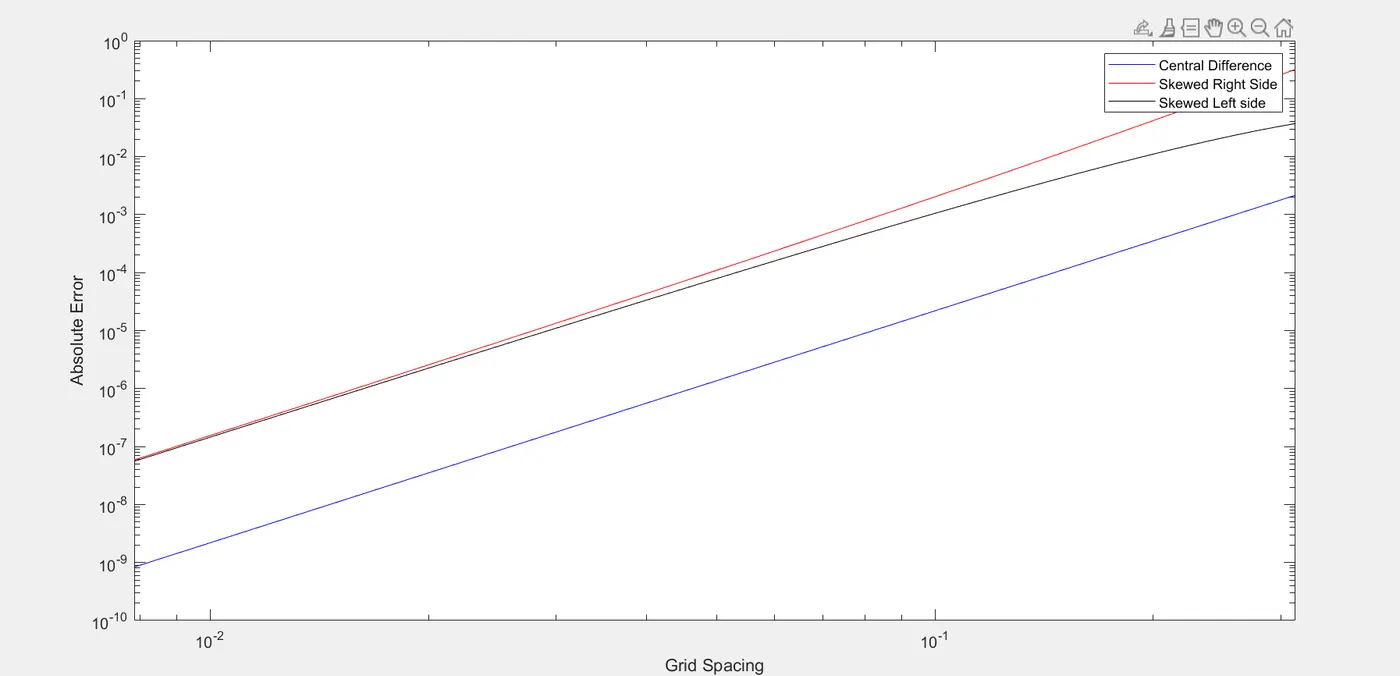
From the above plots we note that the error in a CDS is much less compared to the error in skewed schemes.
However we need to use skewed schemes at the boundary nodes. This is because we do not have grid points either to the right or left of the domain. In such cases we need to use forward or backward differencing schemes.