Week-7 : Converting a detailed engine model to a FRM model
Fast Running Model
Fast Running Engine Model are dynamic, fully physical engine models that are designed specifically to run fast. High fidelity engine models are often too slow running to incorporate system level models where long transient events may be simulated. GT-power engine models can be simplified into FRM using a standard conversion process.
FRMs are able to achieve such fast run times by two means: i) by increasing the simulation time step size, 2) decreasing the number of calculation per time step. These two means are often accomplished at the same time by lumping various flow volumes together which will reduce the total number of subvolumes and also allow for a larger time step size by increasing effective sub volume length.
This report presents series of step followed to convert the tutorial 9 into FRM.
Description of the Model
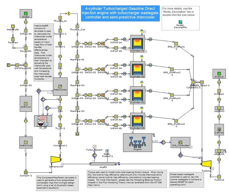
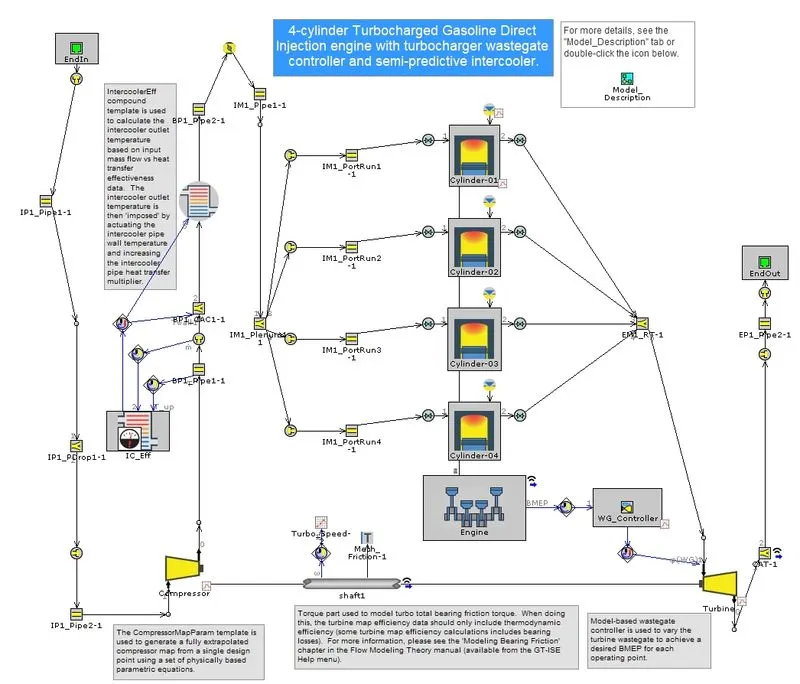
The model which is being considered for analysis is a 4 cylinder-2 liter Turbocharged Gasoline Direct injection engine. It has a turbocharger wastegate controller and semi predictive intercooler. The turbine wastegate is being dynamically controlled in order to target BMEP. A full load speed sweep is being simulated, from 5000 RPM to 1000 RPM. A semi predictive charge air cooler is included such that the outlet temperature is predicted as a function of inlet gas temperature,mass flow rate, coolant temperature and charge air cooler effectiveness.
Conversion Process
1. Step 1-Exhaust Manifold
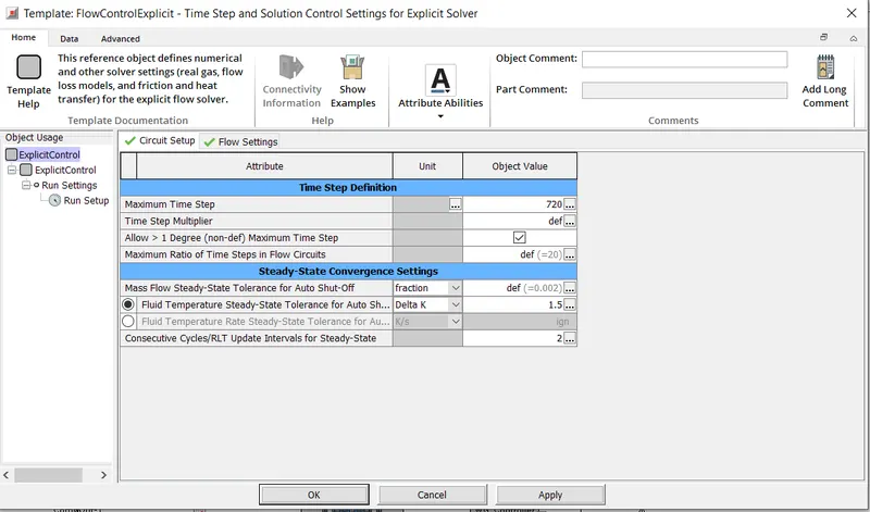
For high fidelity models, the highest gas velocities occur in the exhaust manifold which in turn restricts the time step. Prior to simplification, Maximum Time step was set to 720 as shown below.
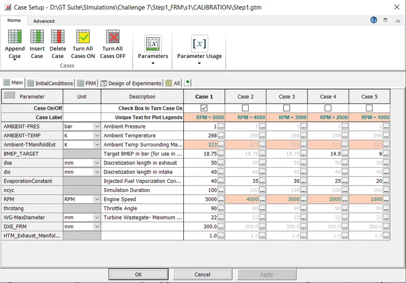
The case setup parameters are shown below
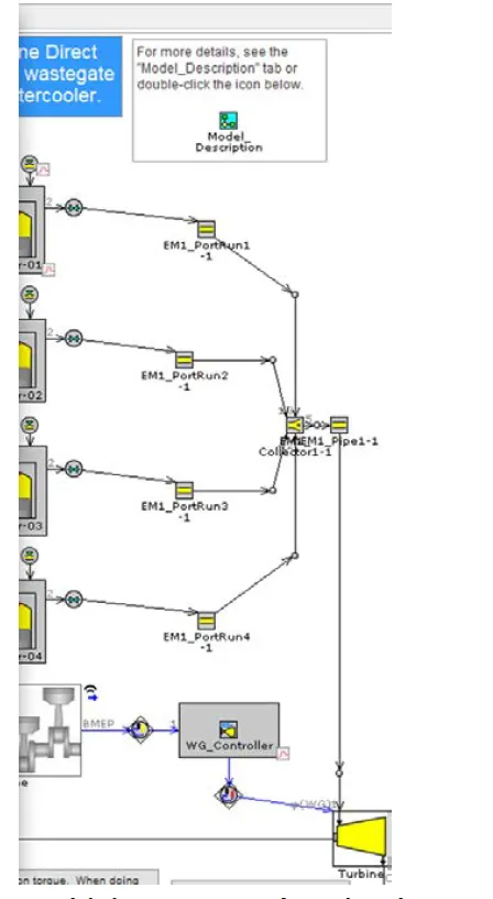
Calibration- Massflow Averaged Inlet Temperature from Turbine part is chosen for calibration.
The lower and upper limit where chosen to be 0.95 and 2.8 respectively.
Step 2: Exhaust Pipes
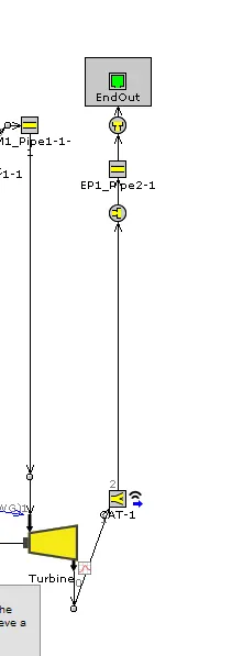
The exhaust pipes downstream of the turbine will be simplified. Three components namely EP1_Pipe1-1, EP1_PDrop1-1 Flowsplit and Orifice Connection between them were selected and Combine Flow Volumes Wizard was launched. This new object was named as CAT.
The newly created CAT1 part was opened and Thermal tab was selected. GasT reference object was selected. Value selector for Wireless Signal or RLT was selected. Value for Exhaust Pipe dia was chosen to be 40mm.
In the calibration RPM 5000 was chosen, Under configure calibration Turbine mass flow averaged outlet pressure was chosen as the parameter. Lower and upper values of exhaust pipes were chosen to be 35mm and 45mm respectively.
Step 3 Intake Manifold
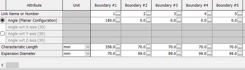
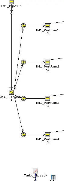
Intake Manifold was selected from FRM convertor and "Simplify for accuracy" option was selected. Modifications were made in the Boundary Data folder of "IM1_Plenum1"
In the Calibration page, case 1 was selected for calibration. Parameter was set to Compressor Massflow Averaged Outlet Pressure.
Step 4:-Compressor Outlet Pipes
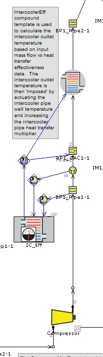
Boost Pipes 1 was selected from Tagged Subsystems list and Simplify for Accuracy was selected.
Intercooler core has been replaced with a FlowSplit and Heat Exchanger connection part. The newly created heat exchange part was selected and Imposed Fluid temperature was set to 300 K. Also in newly created flow split part, Imposed wall temperature was selected and temperature was set to 300 K.
Finally the control links were reconnected.
For the Calibration, case 1 was selected. Parameter selected was Compressor Mass Flow Averaged Outlet Pressure. Lower and upper values for boost pipes was set to 30 and 40mm respectively.
Step 5:- Intake Pipes
Intake Pipes was selected from the Tagged Subsystem list. Simplify for Accuracy selected.
The value of DIA Intake pipe was set to 45 mm. Unused objects were deleted.
In the calibration, Case 1 was selected for calibration. Parameter was set to Compressor Massflow Averaged Inlet pressure. Lower and upper value for intake pipe was set to 40 and 50 mm respectively.
Step 6:- The Exhaust Manifold is selected from FRM converter. "Simplify for speed" is selected
For calibration all cases were enabled for calibration. Turbine Massflow Averaged Inlet Temperature is chosen as the parameter. Lower and Upper values set to 0 and 2.
Step 7:- Cylinder Slaving
This simplification to the model will utilize the Cylinder Slaving capability. The 'slave-RT-full-v2017' was chosen. Cylinder 1 was overriden to master. Each valve was specified as intake or Exhaust valve.
No calibration was chosen for this step, Model was run.
Final FRM model is presented below
FRM Builder approach
In order to calibrate the above model to suite the engine specifications we adopt the FRM Builder tool. The steps followed are
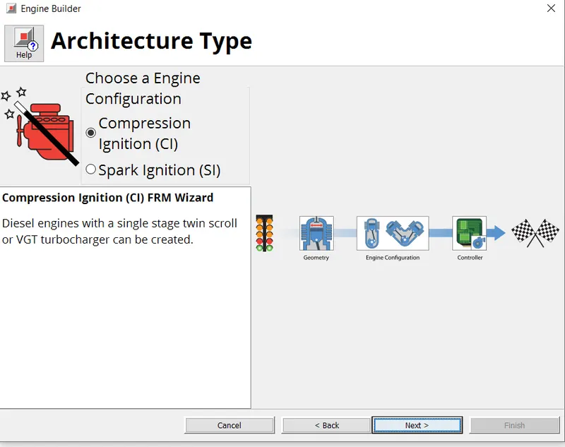
- CI engine selected
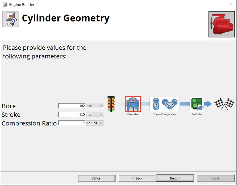
- Engine Bore and stroke set as per the problem statement
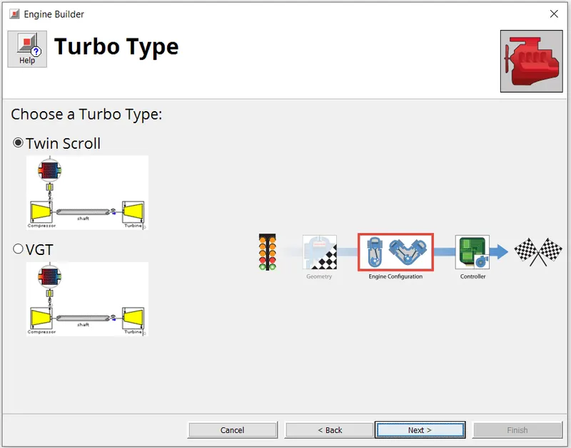
-Twin Scroll Turbo type set
- 6 cylinder engine selected
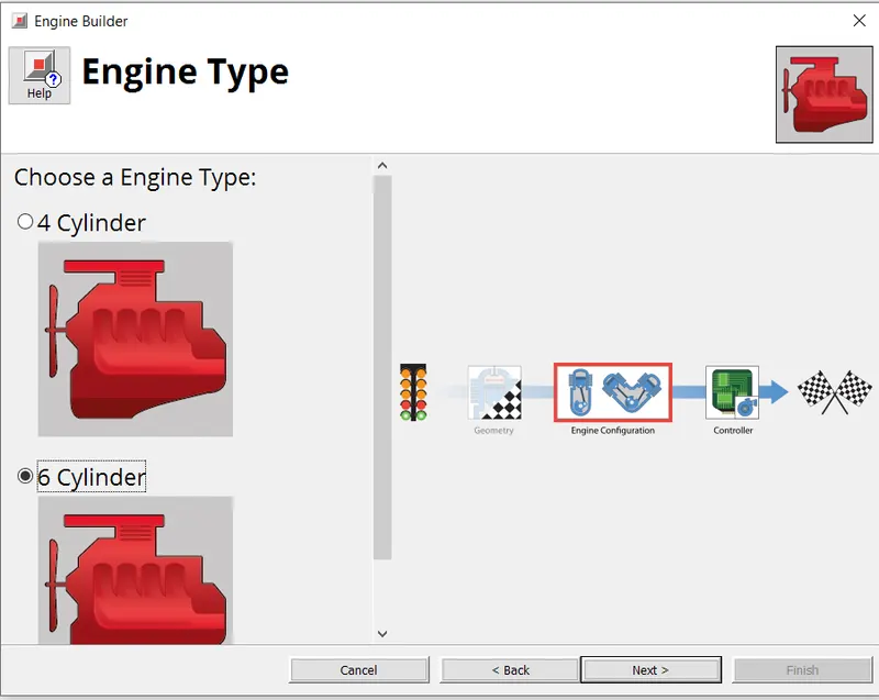
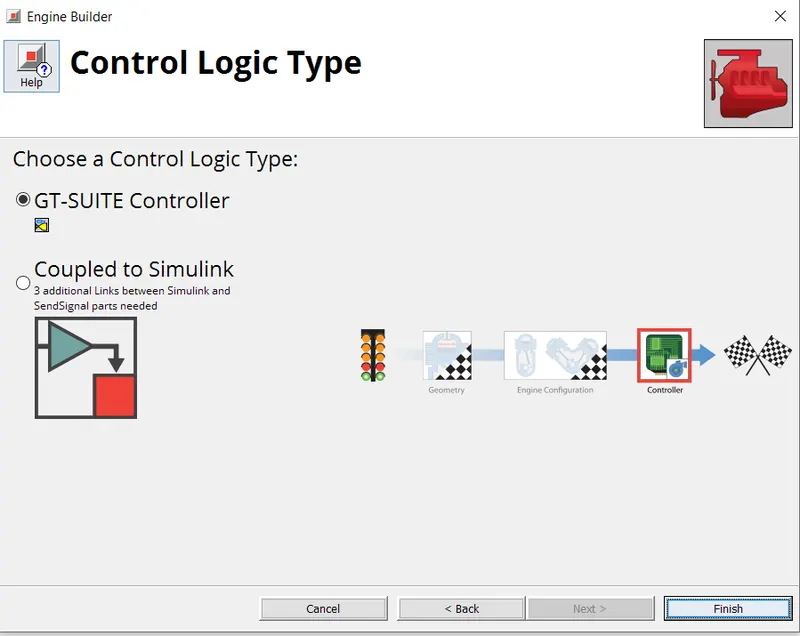
- GT-suite controller selected
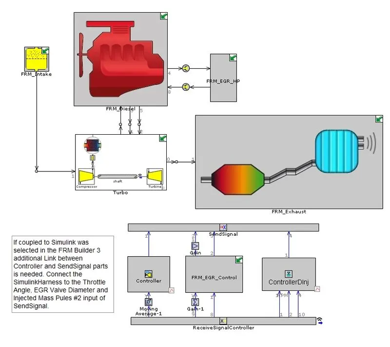
The above steps yield the below FRM model
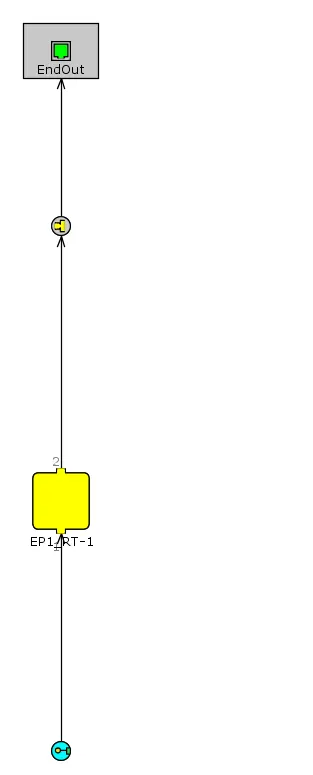
Subcomponents shown below
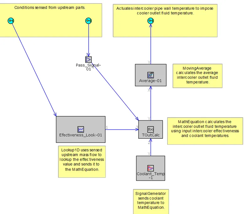
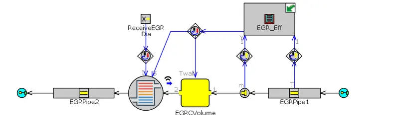
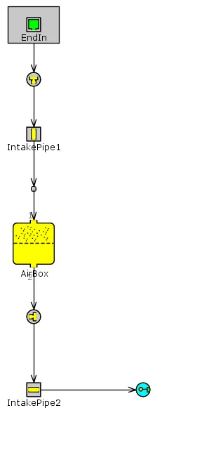
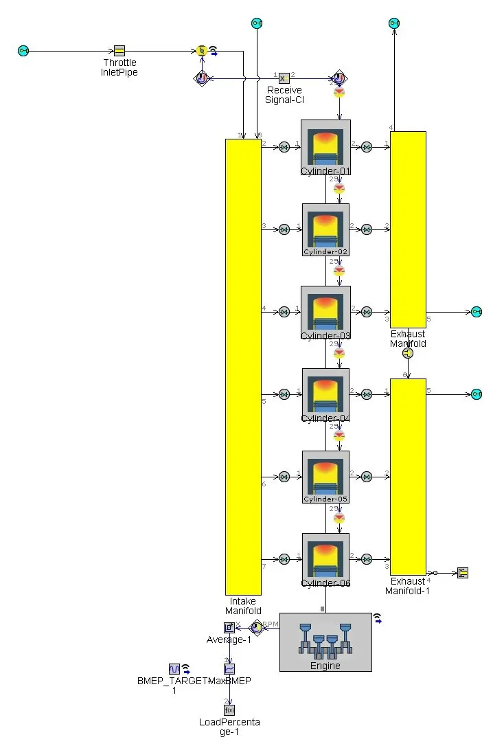
Flow Time comparison
In order to compare the simulation time between FRM and non FRM model, we need to select a suitable base line model. For this purpose the 6 cylinder Turbocharged engine was selected. It yielded the below results
- 6 cylinder Turbocharged Diesel Engine
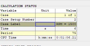
The FRM model for RPM 1500 yields the below result.
-FRM model
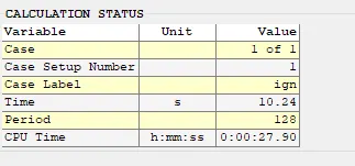
The non FRM model took 6 sec for 75 period wheras FRM took 10.24 for 128 periods. On this count both the models took the same time on an average. However when comparing the CPU time we see that FRM took 27 mins and 90 secs while the non FRM took 1 hr 6mis and 21 sec which is more than double. Therefore FRM is much quicker.
Conclusion:- FRM model was developed for a 4 cylinder turbocharged engine. A seven step process was followed where in high fidelity model was converted into Fast running model. Parts where modified keeping accuracy in mind. The final FRM model was modified as per the required engine specs. Simulation was compared with a baseline model. It was found that FRM model has a significantly less CPU time.