Week 3: Flow over a backward facing step
Aim: The aim of the project is to simulate the flow of air through a backward facing step. The following aspects would be investigated
- Impact of three different mesh sizes would be studied
- Understand the development of flow with the aid of plots for velocity ,pressure and mass flow rate.
Theory:
Backward-Facing Step (BFS) flow is one representative model for separation flows, which can be widely seen in aerodynamic flows (airfoil, spoiler, high attack angle process), engine flows, condensers, vehicles (cars, boat), heat transfer systems, and even the flow around buildings, etc. The flow separation after a simple stage will introduce separation bubble formation, evolution and re-attachment process, which is dependent on the BFS geometric design, the inlet and outlet conditions, turbulent intensity, as well as heat transfer conditions.
The characteristics of a flow over a backward facing step is depicted in the below picture
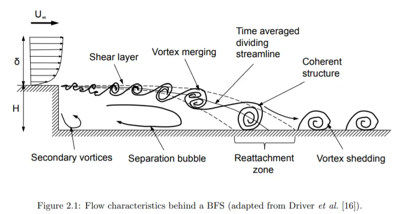
The general characteristics of a BFS flow begins with an upstream boundary layer separating at the step edge due
to the adverse pressure gradient that develops into a thin shear layer. As the flow progresses downstream, the shear layer grows in size with the amalgamation of the turbulent structures contained within. This region where the shear layer develops and grows is referred to as the shear layer region. The turbulent structures in the shear layer entrain irrotational fluid from the non-turbulent region outside the shear layer. This flow entrainment causes the formation of a low velocity recirculation in the region, which is located between the shear layer and the adjacent wall. The recirculation zone is mainly comprised of
a primary vortex in the center and a secondary vortex adjacent to the corner of the step. Due to the favorable pressure gradient created by the fluid entrained,the shear layer eventually curves down towards the wall and impinges at a location known as the reattachment point.
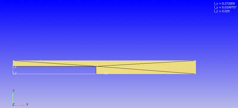
For this analysis, a backward facing step with the below dimensions is considered for the analysis.
Case Setup:-
A. Geometry Creation
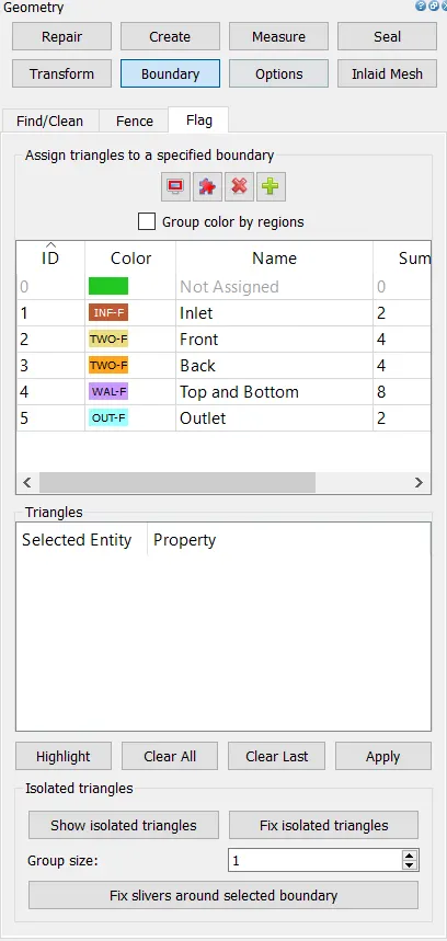
1. Creation of Boundaries: In the geometry which is created above, boundaries such as inflow, outflow , top and bottom walls, front and back faces are labelled.
2. Checking Orientation of Normals: Orientation of Normals were checked to ensure all the normals are pointing inwards. This was done using the Normal Toggle
3. Finally a Diagnosis check was run to ensure no errors in the geometry.
B Case Setup
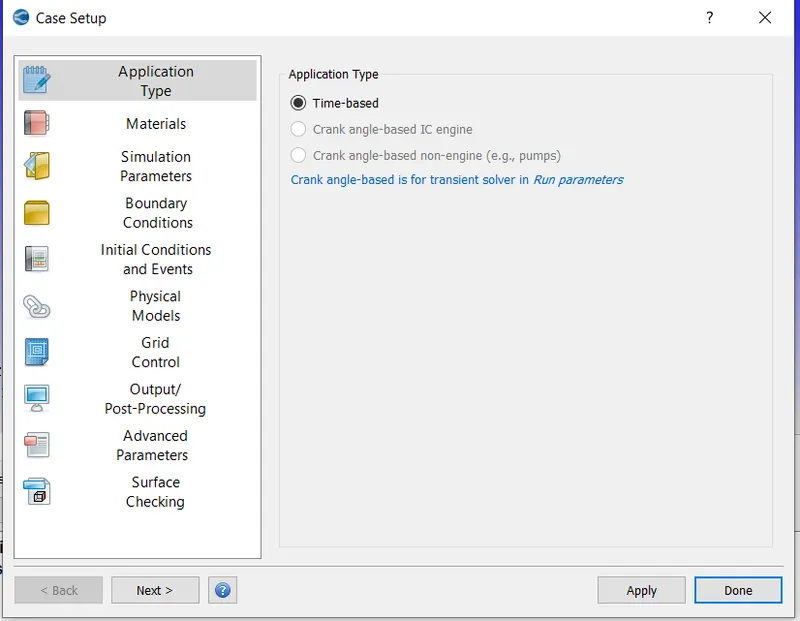
1. Application Type:- This was set to Time based
2.Materials:- This was set to Air
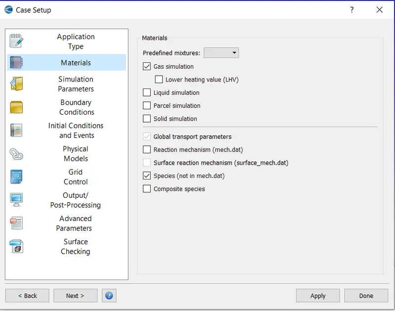
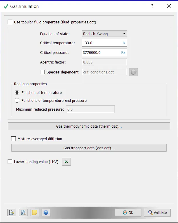
i) Gas Simulation: Default properties were retained
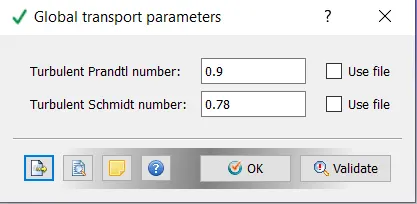
ii) Global Transposrt Parameters:- Default properties retained
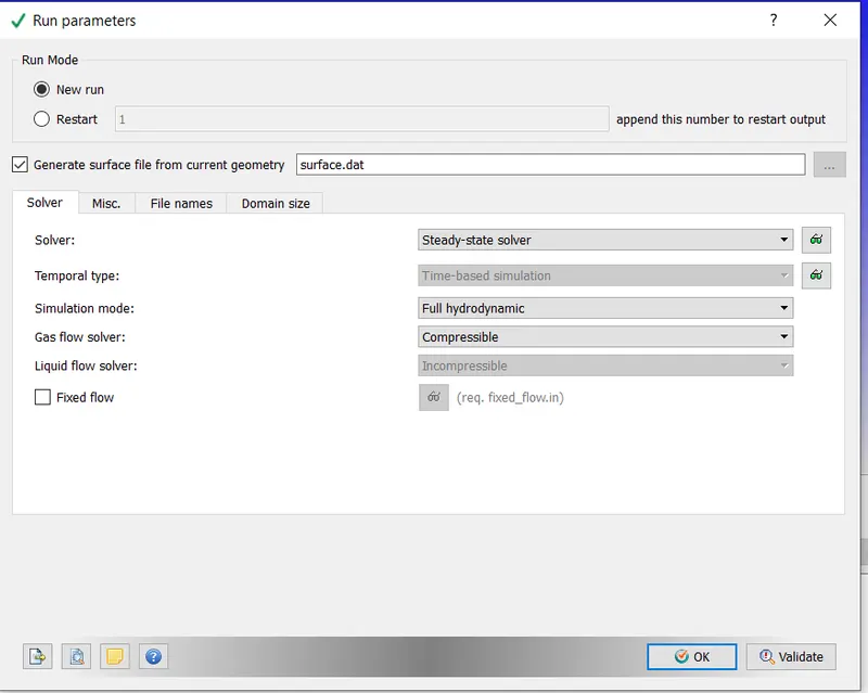
3. Simulation Parameters
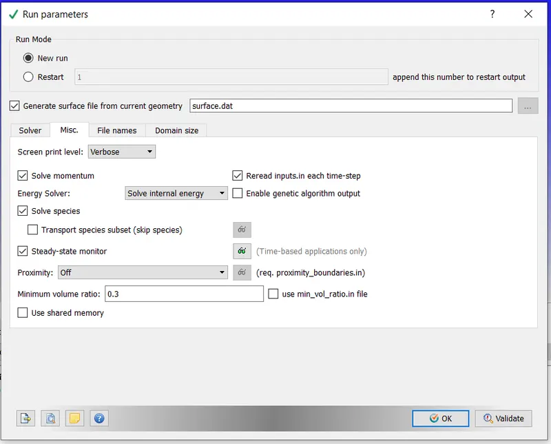
- Run Parameters:- Steady state solver was used. Simulation mode was set to Full Hydrodynamic. Gas Flow solver set to Compressible
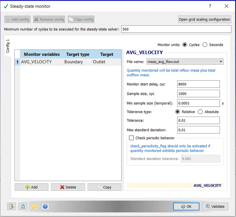
- Steady State Monitor:- Minimum no of cycles for to be executed for Steady state solver -500
Monitor Start Delay, cyc :- 8000
Sample size cyc :- 1000
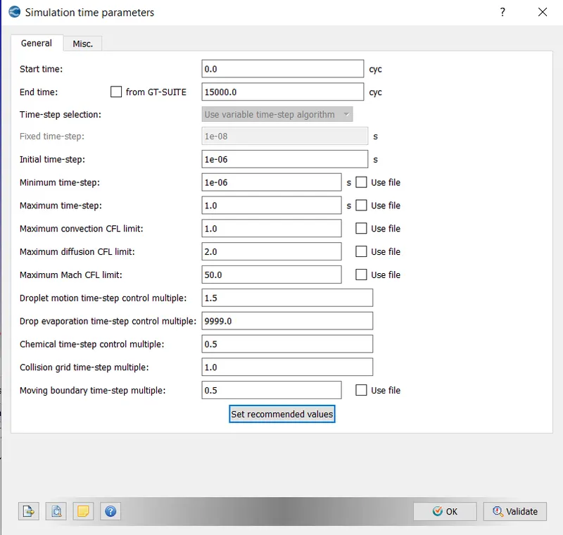
- Simulation Time Parameters:- The parameters were set as displayed below. Max CFL limit set to 1.0
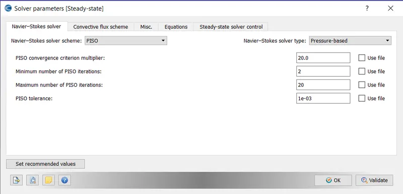
- Solver Parameters:- A Pressure based PISO solver was used, Maximum Convection CFL limit set to 0.8.
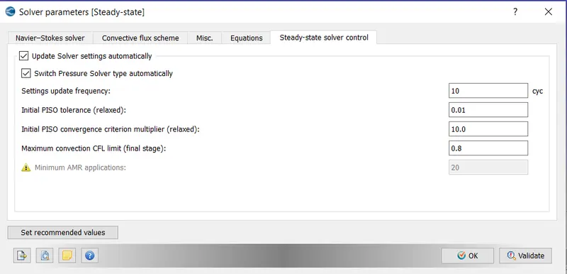
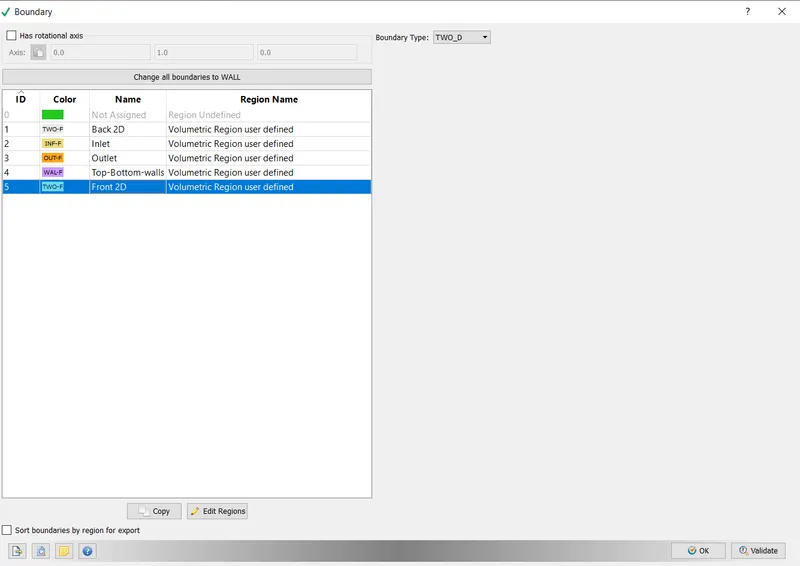
4. Boundary
- Inlet:- Boundary flow - Inflow
Inlet Pressure- 110325 Pa
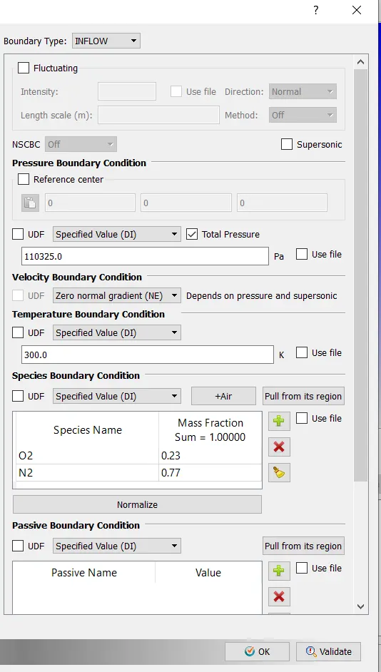
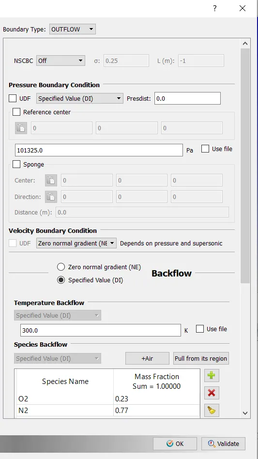
- Outlet- Boundary - Outflow
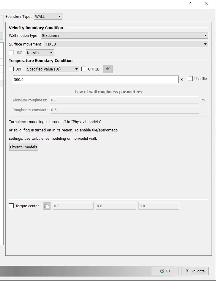
- Top and Bottom Walls:- Stationary wall with Fixed surface movement used
- Front and Back faces set to Two D
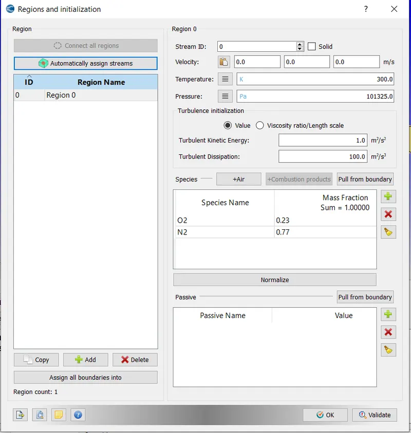
4. Initial condition and events
The created geometry was selected as the Volumetric Region
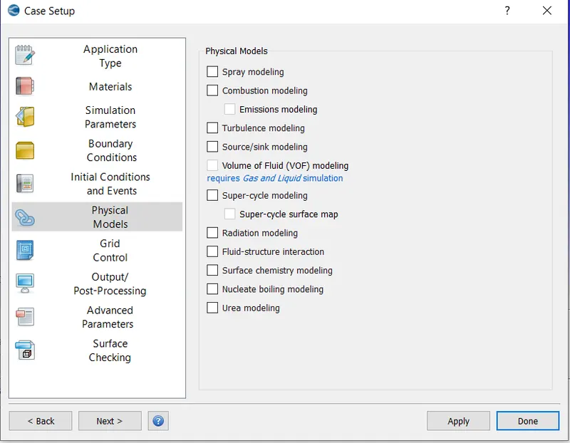
5. Physical Models:- Default retained
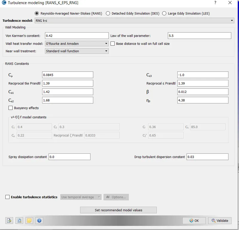
6. Turbulence Modelling:- RNG-kepsilon turbulence model is used
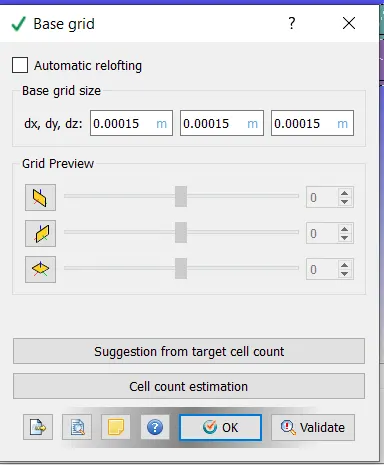
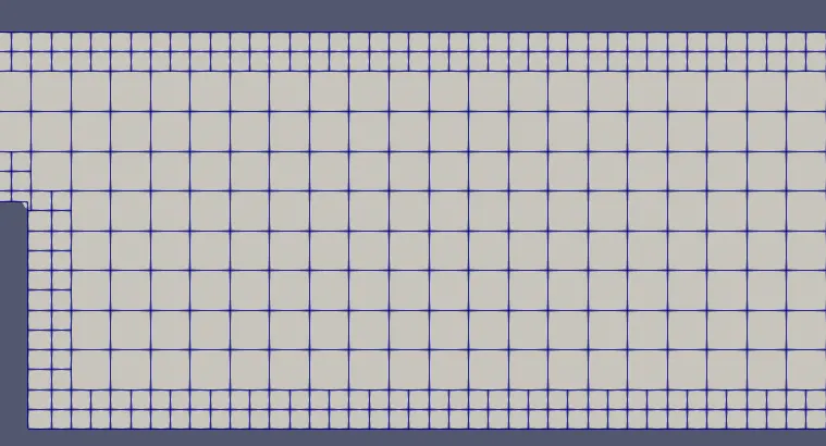
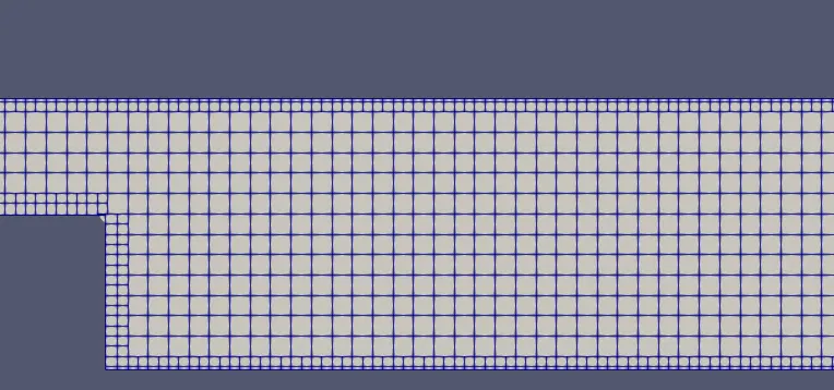
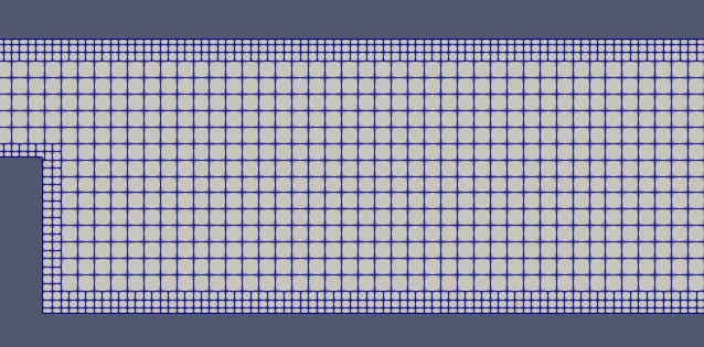
7. Grid Control:- Base Grid. Here the size of the mesh for the three cases is entered
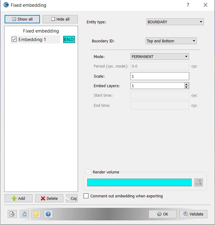
Fixed Embedding was also enabled
This feature is used to refine the grid at specific locations in the domain where a finer resolution is critical to the accuracy of the solution.
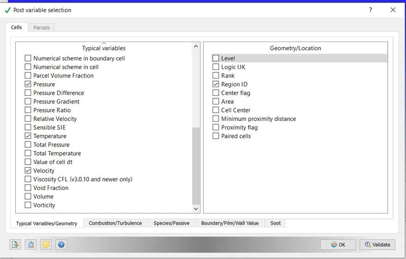
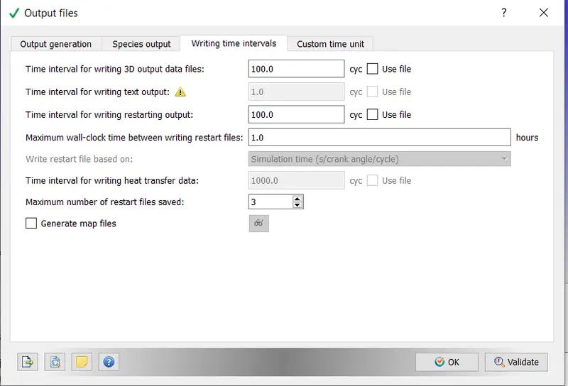
7. Output/Post Processing:- The variables that we intend to see during post processing are selected. In this case Density, Pressure , Temperature and Velocity were selected.
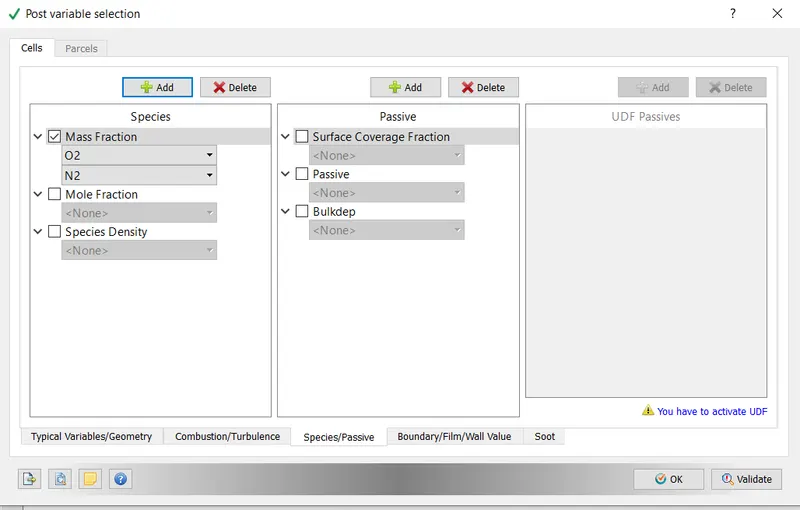
Also the frequency of generation of output files were set below
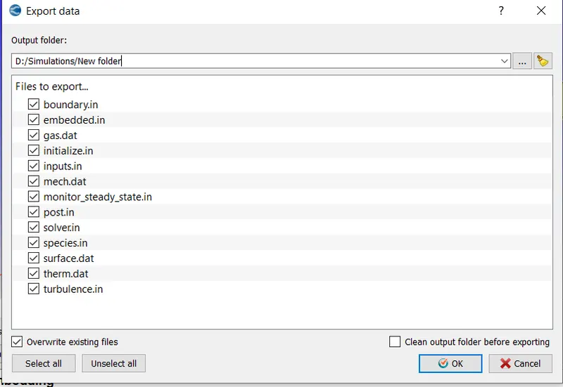
After setting the above, the input files were exported to a directory
In order to execute the simulation, the directory in which these input files were stored was accessed in Cygwin and the following command was typed "mpiexec.exe -n 4 converge.exe"
After the Simulation was executed, the results were converted into a form which would be compatible with Paraview. This was done using the post_convert.exe command.
Results and Post Processing
i) Case 1 (Mesh Size 2e-03)
a) Structure of Mesh

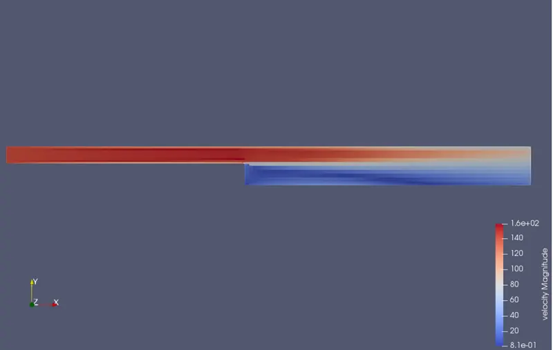
b) Velocity Contour
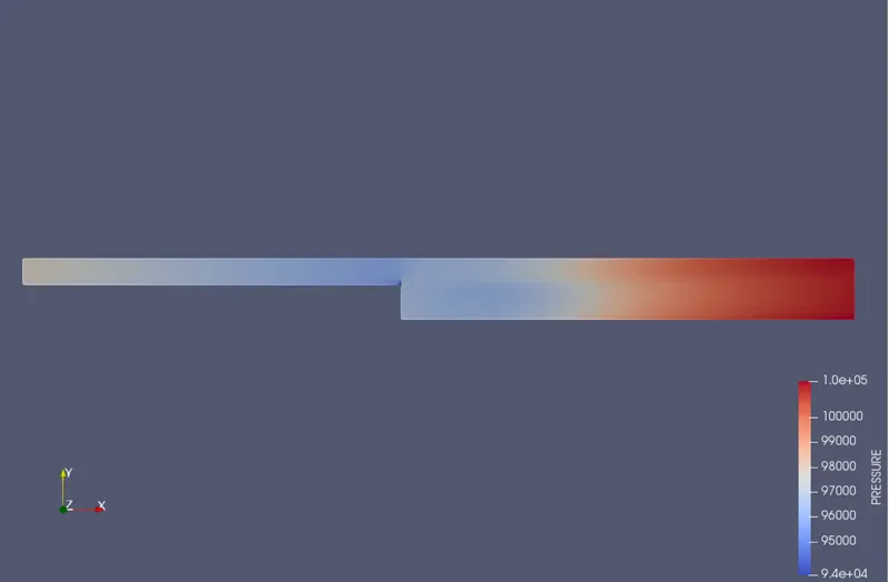
ii) Pressure Contour
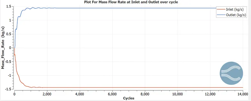
iii) Plots at inlet and outlet during Computational Cycle
- Mass Flow Rate
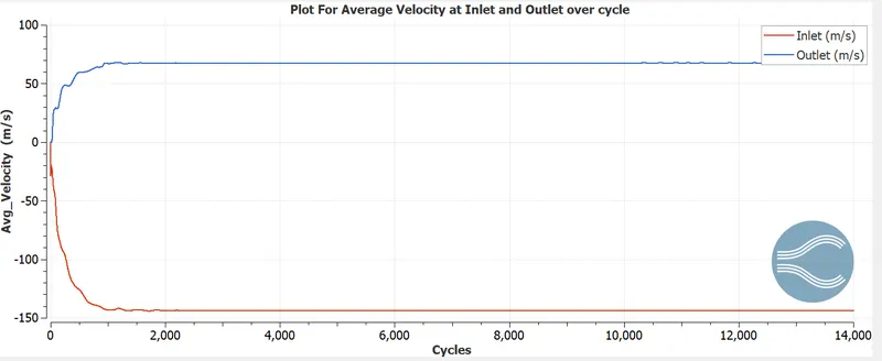
- Average Velocity
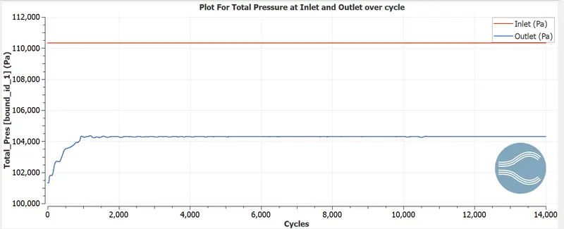
- Total Pressure
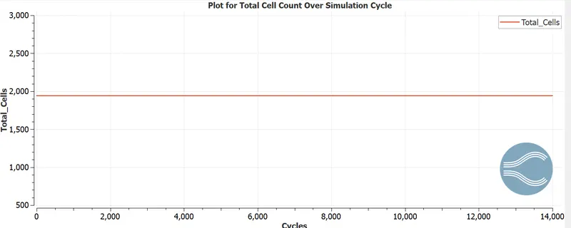
- Cell Count
ii) Case 2 (Mesh Size 1.5e-03)
a) Structure of Mesh

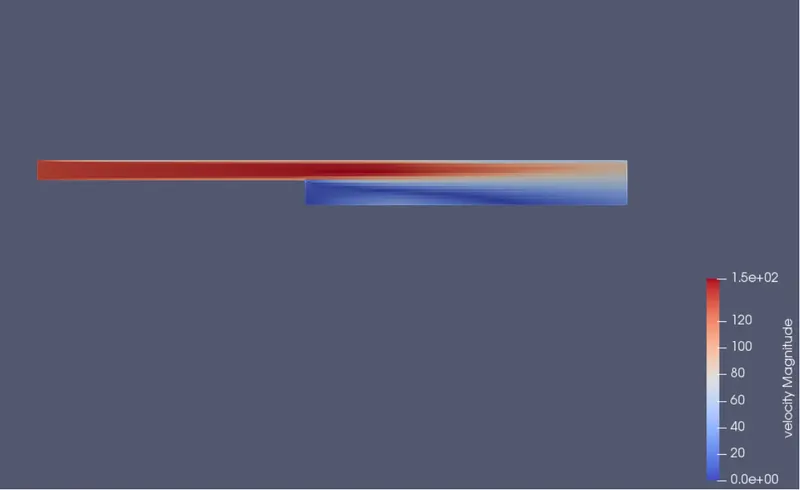
b) Velocity Contour
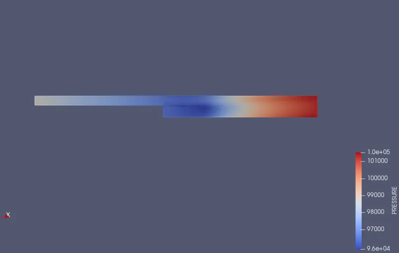
ii) Pressure Contour
iii) Plots at inlet and outlet during Computational Cycle
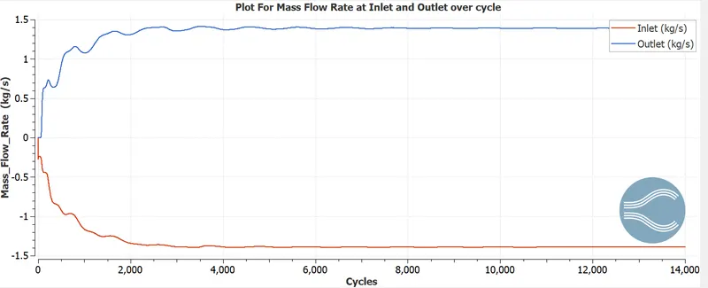
- Mass Flow Rate
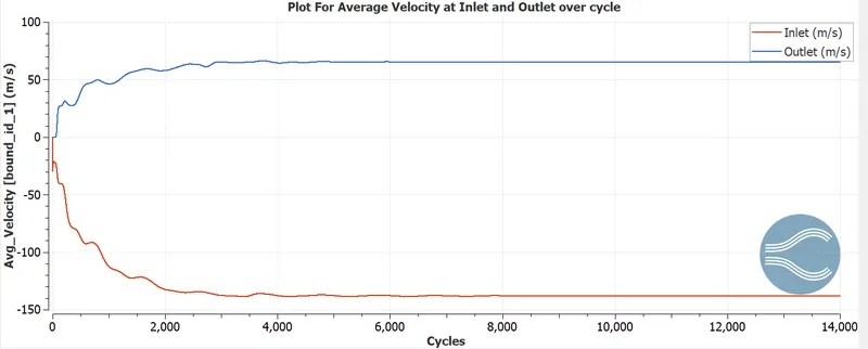
- Average Velocity
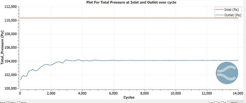
- Total Pressure
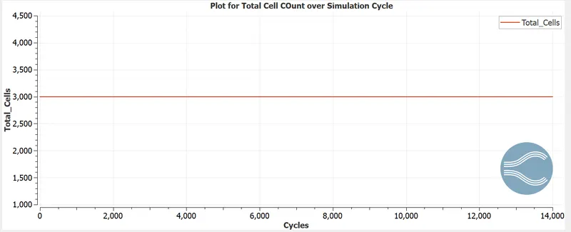
- Cell Count
iii) Case 2 (Mesh Size 1.2e-03)
a) Structure of Mesh

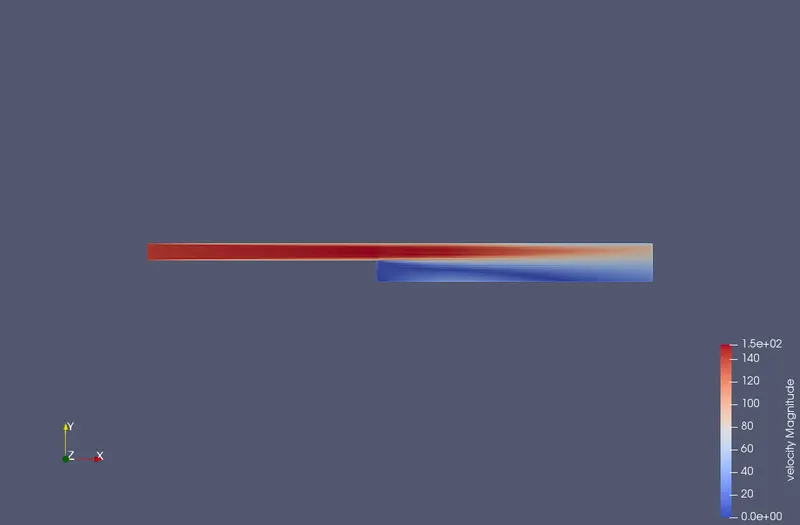
b) Velocity Contour
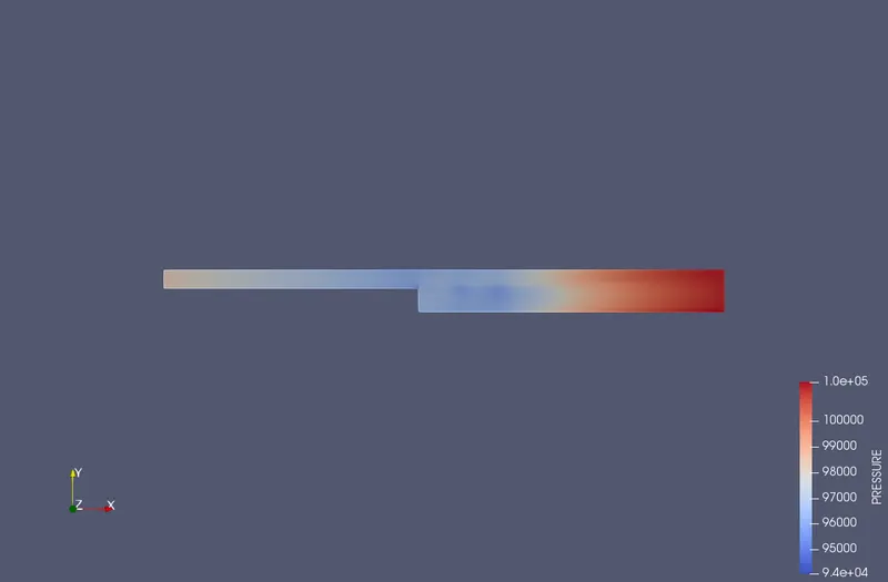
ii) Pressure Contour
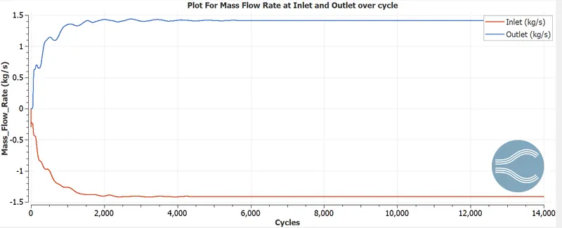
iii) Plots at inlet and outlet during Computational Cycle
- Mass Flow Rate
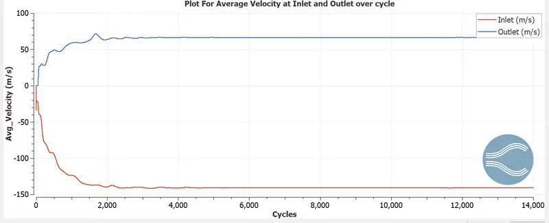
- Average Velocity
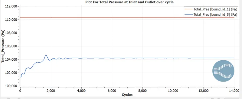
- Total Pressure
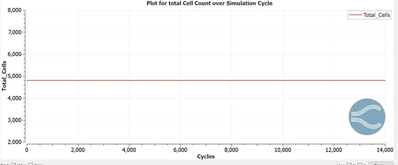
- Cell Count
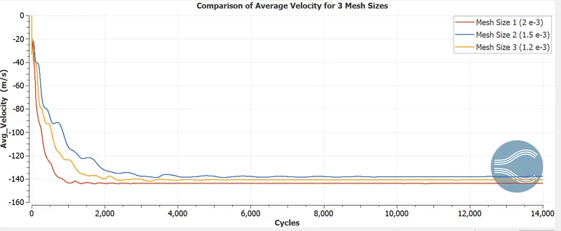
Comparison of Velocity and Mass flow rates for Different Mesh Sizes
Velocity
i) Inlet
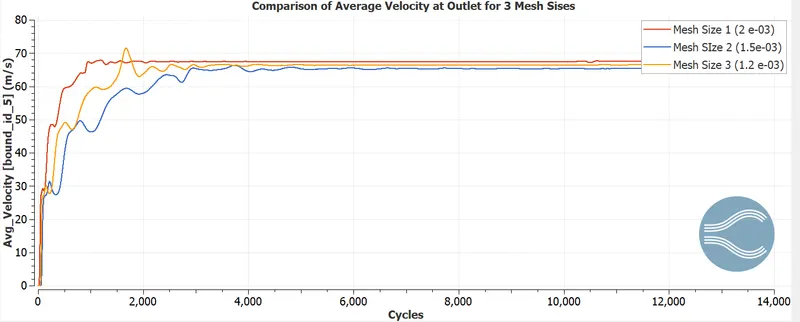
ii) Outlet
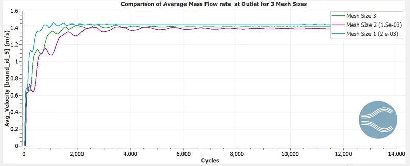
Mass Flow Rate
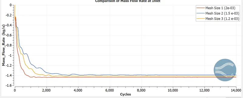
- Inlet
-Outlet
Animations
i) Velocity
- Case 1 ( Mesh Size 2.0 e-3)
https://www.youtube.com/watch?v=mlBVWp0JI8Q&ab_channel=VivekRamesh
- Case 2 ( Mesh Size 1.5 e-3)
https://www.youtube.com/watch?v=rxhY05pzkdU&ab_channel=VivekRamesh
- Case 3 (Mesh Size 1.2 e-3)
https://www.youtube.com/watch?v=8XTOeGIUDxg&ab_channel=VivekRamesh
ii) Pressure
- Case 1 ( Mesh Size 2.0 e-3)
https://www.youtube.com/watch?v=S22mqEiypQk&ab_channel=VivekRamesh
- Case 2 ( Mesh Size 1.5 e-3)
https://www.youtube.com/watch?v=00y-ZS7Uszk&ab_channel=VivekRamesh
- Case 3 (Mesh Size 1.2 e-3)
https://www.youtube.com/watch?v=GG_WL6UJIac&ab_channel=VivekRamesh
Observations
The Following inferences can be drawn from the above plots
1. The driving force for the flow is the variation in pressure between inlet and outlet.
2. The flow at the inlet is around 150 m/s. As it flows through the step the area increases resulting in a loss of velocity. This reduction in velocity can be expressed by the continuity equation Area*Velocity=constant.
3. From the velocity contour, we can also observe that in the step region there is an area where flow velocity drops to zero. Flow separates as a result of adverse pressure gradient. However, The turbulent structures in the shear layer entrain irrotational fluid from the non-turbulent region outside the shear layer. This flow entrainment causes the formation of a low velocity recirculation in the region, which is located between the shear layer and the adjacent wall. The recirculation zone is mainly comprised ofa primary vortex in the center and a secondary vortex adjacent to the corner of the step. Due to the favorable pressure gradient created by the fluid entrained,the shear layer eventually curves down towards the wall and impinges at a location known as the reattachment point.
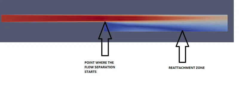
3. From the pressure plot initially we observe that the pressure is high at the inlet and it goes on increasing till it reaches the step region. After the reattachment point the pressure increases until the outlet
4. From the mass, velocity and total pressure plots we observe that after about 4000 cycles it reaches a steady state and there is no variation in the values. From the animations to we observe that after 25 seconds the solution converges to its steady state value.
5. Minor variations are observed in the values of mass flow rates, average velocity etc during the course of simulation.
5. The cell count remains a constant during the course of the computational cycle