Week 5.2 - Literature review: ODE Stability

Aim:- The aim of this exercise is to understand the stability of an ODE system

When does a ODE become unstable?

Consider the following two dimensional system:

`dotx=f(x,y)`

`doty=g(x,y)`

and suppose that `(barx,bary)`is a steady state, that is

`f(barx,bary)=0`

`g(barx,bary)=0`

Consider a small pertubation from the steady state by letting

`x=barx+u`

`y=bary+v`

where both u and v are understood to be small. The question of interest is whether u and v will grow (away from steady state) or will they decay to zero (reach steady state).

Deriving differential equations for u and v

`dotu=dotx`

=`f(x,y)`

=`f(barx+u,bary+u)`

=`f(barx,bary) + (delf)/(delx)(barx,bary)u + (delf)/(dely)(barx,bary)v +........` (Taylor series expansion)

=`(delf)/(delx)(barx,bary)u + (delf)/(dely)(barx,bary)v`(since `f(barx,bary)'=0, steady state )

Similarly

`barv=(delg)/(delx)(barx,bary)u + (delg)/(dely)(barx,bary)v`

Neglecting higher order terms we obtain the following linear system of equations

`((dotu),(dotv))=(((delf)/(delx)(barx,bary),(delf)/(dely)(barx,bary)),((delg)/(delx)(barx,bary),(delg)/(dely)(barx,bary)))(u,v)`

The matrix is referred to as Jacobian matrix of the original system at steady state (u,v)=(0,0)

The above linear sytem for u and v has the trivial steady state (u,v)=(0,0) and the stability of this trivial steady state is determined by eigenvalues of the matrix as follows

- If eigenvalues of the jacobian matrix all have real parts less than zero, the steady state is stable

- If at least one of the eigenvalues of the Jacobian matrix has real part grater than zero, the steady state is unstable

- Otherwise there is no conclusion. It is a borderline case between stability and instability. This requires advanced mathematical analysis to determine stability.

Applying the above principle to the Eulers Method

-Forward Eulers

`y_(k+1)=y_k + h*f(t_k,y_k)`

For an ODE `dy/dt=lambday` with `y(0)=y_0`

`y_(k+1)= y_k +hlambday_k`

`y_(k+1)= y_0(1 +hlambda)^(k+1)`

The forward Euler method is stable if

`|1+hlambda|<= 1`

Similarly The Backward Euler method is stable if

`1/|1+hlambda|<= 1`

for real `lambda' `1/|1+hlambda` is lesser than one so the system is unconditionally stable

To gain an understanding of the above methods we consider the following function

`(dy)/(dt)= -1000y-e^(-t)`

- Explicit Formulation

`y^(n+1)=y^n-1000y^n*Deltat-e^-t.(Deltat)`

comparing it with our standard formulation, we note that

`lambda=-1000`, `h=Deltat`

Condition for expicit formulation to be stable is given by

`|1+hlambda|<= 1`

This implies

`hlambda<= 0` (trivial condition)

`-1-hlambda>=1`

`hlambda <= -2'

`h<=-2/lambda`

or ' Deltat<=-2/-1000'

`Deltat<=0.002'

We can infer that the explicit scheme will be stable if the timestep is smaller than or equal to 0.002.

- Implicit formulation

`y^n=(-1000y^n-e^-t)(Deltat) +y^(n-1)`

Solving for `y^n`

`y^n=(y^(n-1)-e^(-t)Deltat)/(1+1000*(Deltat)`

- Analytical Solution (from Wolfram Alpha)

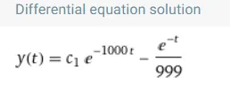
xWe compute the analytical, implicit and explicit solution with the help of a Python Program

import numpy as np
import matplotlib.pyplot as plt
import math

def analytical(t_tot,dt):
    t=np.arange(0,t_tot,dt)
    y=np.zeros(len(t))
    for i in range(0,len(t)):
        y[i]=math.exp(-1000*t[i])*(1-math.exp(999*t[i]))/999
    return[t,y]
def explicit(t_tot,dt):
    t=np.arange(0,t_tot,dt)
    y=np.zeros(len(t))
    for i in range(0,len(t)):
        y[i]=y[i-1]+ dt*(-1000*y[i-1]-np.exp(-t[i-1]));
    return[t,y]
def implicit(t_tot,dt):
    t=np.arange(0,t_tot,dt)
    y=np.zeros(len(t))
    for i in range(0,len(t)):
        y[i]=(y[i-1]- np.exp(-t[i])*dt)/(1+1000*dt)
    return[t,y]

t_tot=0.5
dt=0.0009
t,y_ana = analytical(t_tot,dt)
t,y_exp = explicit(t_tot,dt)
t,y_imp=implicit(t_tot,dt)

plt.plot(t,y_ana)
plt.plot(t,y_exp) 
plt.plot(t,y_imp)
plt.legend(["analytical","explicit", "implicit"])
plt.grid('on')
title=('timestep: ',dt)
plt.show()

As stated earlier explicit solution is stable if time step is smaller or equal to 0.002

- dt 0.0009

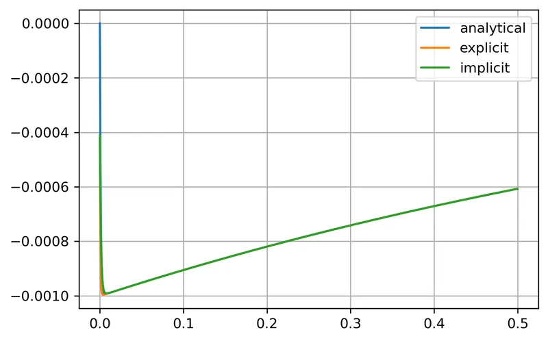
We can see from the above plot that there is a good agreement between three methods

- dt=0.0019

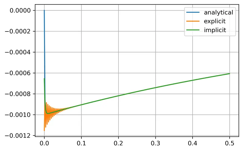
at dt=0.0019 we see that there is good agreement between three methods, however some oscillations are observed in the explicit method

-0.0025

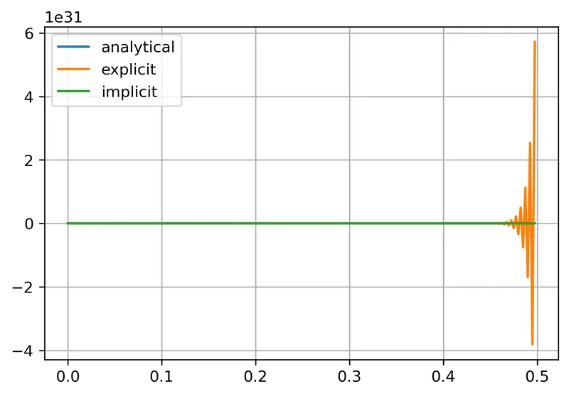
at dt= 0.0025 magnitude of oscillations for explicit method has increased.

-0.008

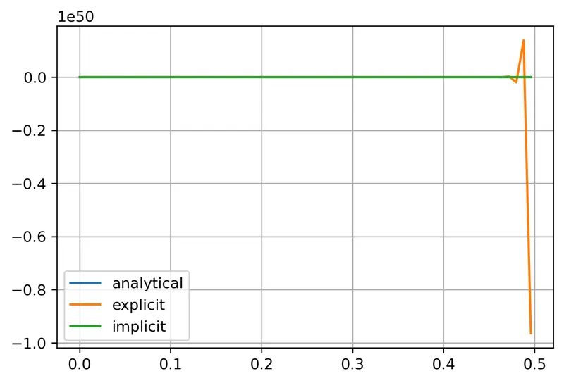
It is noted that the explicit solution has completely blown up.

How does stability affect engineering simulations

Stability refers to the sensitivity of the solution to pertubations of the initial values. An ODE is called unstable if pertubations grow with time and errors get magnified. Instabilility in numerical solutions results in obtaining unphysical and impractical results. Moreover computational resources to are wasted by setting numerical unstable schemes.

Can stability condition be derived for all types of problems?

Stability can only be derived if eigen values of the Jacobian Matrix have real parts less than zero.If atleast one of the eigen values have real part greater than zero, equation is unstable.

If the eigen values do not satisfy any of the above criteria, it is neutrally stable and no stability criteria can be obtained explicitly.