Week 7 - Auto ignition using Cantera
Aim:-The aim of this challenge is to simulate the auto ignition temperature for methane under the following conditions
- constant temperature of 1250K and pressure varying from 1 to 5 atm.
- constant pressure of 5 atm and temperature varying from 950K to 1450K.
-observe and print the rate of change of molar concentrations of the given elements "H2O, O2, OH" with respect to the time
Auto ignition:- Autoignition occurs when a mixture of gases or vapors ignites spontaneously with no external ignition source and after reaching a certain temperature, the autoignition temperature. The autoignition temperature is not an intrinsic property of the gases or vapors but is the lowest temperature in a system where the rate of heat evolved from the gases or vapors increases beyond the rate of heat loss to the surroundings, resulting in ignition. The autoignition temperature of a mixture of gases or vapors is affected by pressure, vessel shape and volume, surface activity, contaminants, flow rate, reaction rate, droplet and mist formation, gravity, and reactant concentration.
Ignition Delay:- The period between the beginning of fuel injection into an engine cylinder and the begining of combustion is called ignition delay. The delay period consists of a physical delay,where in atomization,vaporization and mixing of air fuel occur and of chemical delay attributed to pre combustion reactions. Reducing NOx in modern engine is achieved via reducing ignition delay.
Governing Equations for Single reactors
The state variables in general reactor model are
- mm, mass of reactors contents
- VV the reactor volume in m^3
- State variable describing the energy of the system depending on the configuration
- General Reactor:UUm the total internal energy of the reactor contents
- Const Pressure Reactor. HH, the total enthalpy of the reactor contents
- IdealGasReactor: TT, the temperature in K
- Ideal GasConstPressureReactor
- Mass fractions of each species
Mass Conservation
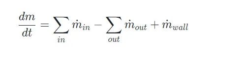
The total mass of the reactor's contents changes as a result of flow through the reactor's inlets and outlets, and production of homogeneous phase species on the reactor walls
Species Conservation
The rate at which species kk is generated through homogeneous phase reactions is V \dot{\omega}_k W_kVω˙kWk, and the total rate at which species kk is generated is
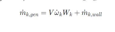
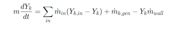
The rate of change in the mass of each species is:

Expanding the derivative on the left hand side and substituting the equation for dm/dtdm/dt, the equation for each homogeneous phase species is:
Reactor Volume
The reactor volume changes as a function of time due to the motion of one or more walls:
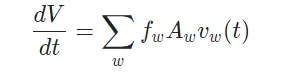
where f_w = \pm 1fw=±1 indicates the facing of the wall (whether moving the wall increases or decreases the volume of the reactor), A_wAw is the surface area of the wall, and v_w(t)vw(t) is the velocity of the wall as a function of time.
For the ConstPressureReactor() and IdealGasConstPressureReactor(), the volume is not a state variable, but instead takes on whatever value is consistent with holding the pressure constant
The solution of the energy equation can be enabled or disabled by changing the energy_enabled flag. It is enabled by default.
The implemented formulation of the energy equation depends on which reactor model is used.
Standard Reactor
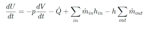
The equation for the total internal energy is found by writing the first law for an open system:
Constant Pressure Reactor
For this reactor model, the pressure is held constant. The volume is not a state variable, but instead takes on whatever value is consistent with holding the pressure constant. The total enthalpy replaces the total internal energy as a state variable. Using the definition of the total enthalpy:
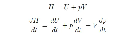
Noting that dp/dt = 0dp/dt=0 and substituting into the energy equation yields:

Ideal Gas Constant Pressure Reactor

import matplotlib.pyplot as plt
import cantera as ct
import numpy as np

gas=ct.Solution('gri30.xml')
temp=np.linspace(950,1450,11)

t_start=0
t_end=10
time_step=1e-3
n=int((t_end-t_start)/(time_step))
temp=np.linspace(950,1450,11)
ign_delay_T=[]
states1=[]
for i in temp:
    gas.TPX=i,5*101325,{'CH4':1,'O2':2,'N2':7.52}
    T_ai=0
    t_ai=0
    time=0
    r=ct.IdealGasReactor(gas)
    sim=ct.ReactorNet([r])


    states=ct.SolutionArray(gas,extra=['t_ms','t'])
   # print('{:10s}{:10s}{:10s}'.format('t[s]','T[K]','P[Pa]'))
    for n in range(n):
        time+=1e-3
        sim.advance(time)
        states.append(r.thermo.state, t_ms=time*1e3,t=time)
        #print('{:10.3e}{:10.3f}{:10.3f}'.format(sim.time,r.T,r.thermo.P))
    states1.append(states.T)

    for i in range(n):
        T_error=states.T[i]-i-400

        if T_error>0:
            T_ai=states.T[i]
            t_ai=states.t_ms[i]
            break
    ign_delay_T.append(t_ai)

state1=np.array(states1)

for k in range(len(temp)):
    plt.figure(1)
    plt.plot(states1[k])
    plt.xlabel('Number of timesteps')
    plt.ylabel('Temperature')
    plt.title('Variation of Auto-ignition Time with inlet pressure')
    plt.legend(['1 Bar', '1.5 Bar','2 Bar','3 Bar','3.5 Bar','4 Bar','4.5 Bar','5 Bar'])

plt.figure(2)
plt.savefig('Time Delay vs temp @ const p', dpi=300, bbox_inches='tight')
plt.plot(pressure,ign_delay_P )
plt.xlabel('Pressure[bar]')
plt.ylabel('Auto-ignition Time[ms]')
plt.title('Ignition time delay vs temp')
plt.show()
In the above code gas is assumed to be at 1250 K. Program is to be run for 10 seconds with a time step of 1ms. Nine values of pressure has been specified from 1 bar to 5 bar using linspace command.
The below criteria is used to define the ignition delay time.

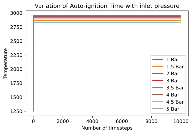
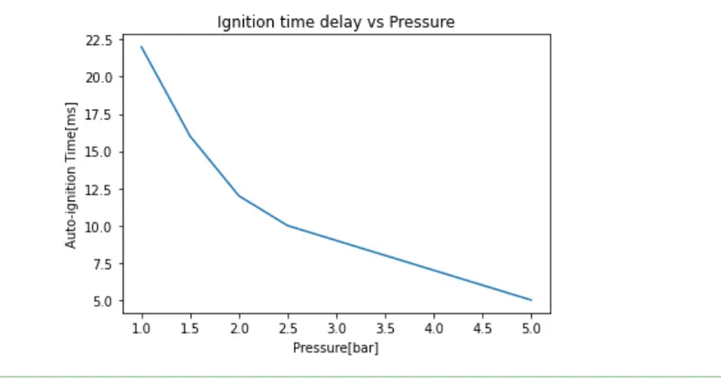
It can be seen that for a low pressure reactor ignition delay is high and for a high pressure reactor ignition delay is low. The maximum flame temperature reached by products is maximum for a high pressure reactor and low for a low pressure reactor.
Ignition delay is maximum for a low pressure reactor and minimum for a high pressure reactor. high pressure facilitates auto ignition and helps mixture burn faster.
Auto Ignition For Varying Temperature
import matplotlib.pyplot as plt
import cantera as ct
import numpy as np

gas=ct.Solution('gri30.xml')
temp=np.linspace(950,1450,11)

t_start=0
t_end=10
time_step=1e-3
n=int((t_end-t_start)/(time_step))
temp=np.linspace(950,1450,11)
ign_delay_T=[]
states1=[]
for i in temp:
    gas.TPX=i,5*101325,{'CH4':1,'O2':2,'N2':7.52}
    T_ai=0
    t_ai=0
    time=0
    r=ct.IdealGasReactor(gas)
    sim=ct.ReactorNet([r])


    states=ct.SolutionArray(gas,extra=['t_ms','t'])
   # print('{:10s}{:10s}{:10s}'.format('t[s]','T[K]','P[Pa]'))
    for n in range(n):
        time+=1e-3
        sim.advance(time)
        states.append(r.thermo.state, t_ms=time*1e3,t=time)
        #print('{:10.3e}{:10.3f}{:10.3f}'.format(sim.time,r.T,r.thermo.P))
    states1.append(states.T)

    for i in range(n):
        T_error=states.T[i]-i-400

        if T_error>0:
            T_ai=states.T[i]
            t_ai=states.t_ms[i]
            break
    ign_delay_T.append(t_ai)

state1=np.array(states1)
for k in range(len(temp)):
    plt.figure(1)
    plt.savefig('Autoig vs temp.png', dpi=300, bbox_inches='tight')
    plt.plot(states1[k])
    plt.xlabel('Number of timesteps')
    plt.ylabel('Temperature')
    plt.title('Variation of Auto-ignition Time with inlet pressure')
    plt.legend(['950K', '1000K','1050K','1100K','1150K','1200K','1250K','1300K','1350K','1400K','1450K'])


plt.figure(2)
plt.savefig('Time Delay vs temp @ const p.png', dpi=300, bbox_inches='tight')
plt.plot(pressure,ign_delay_P )
plt.xlabel('Pressure[bar]')
plt.ylabel('Auto-ignition Time[ms]')
plt.title('Ignition time delay vs temp')
plt.show()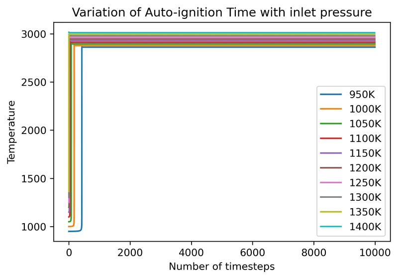
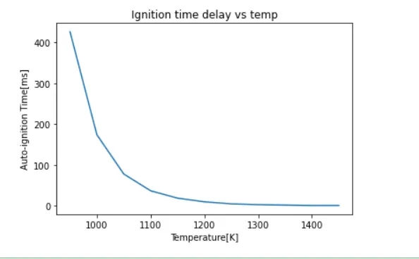
It can be seen that for a high initial temperaturem the auto ignition delay time is least.Final temperature achieved after ignition is highest when initial temperature is high.
Ignition delay is maximum for a low temperature reactor and minimum for a high temperature reactor. high temperature facilitates auto ignition and helps mixture burn faster.
import matplotlib.pyplot as plt
import cantera as ct
import numpy as np

gas=ct.Solution('gri30.xml')
temp=np.linspace(950,1450,11)

t_start=0
t_end=10
time_step=1e-3
n=int((t_end-t_start)/(time_step))
temp=np.linspace(950,1450,11)
ign_delay_T=[]
states1=[]
for i in temp:
    gas.TPX=i,5*101325,{'CH4':1,'O2':2,'N2':7.52}
    T_ai=0
    t_ai=0
    time=0
    r=ct.IdealGasReactor(gas)
    sim=ct.ReactorNet([r])


    states=ct.SolutionArray(gas,extra=['t_ms','t'])
   # print('{:10s}{:10s}{:10s}'.format('t[s]','T[K]','P[Pa]'))
    for n in range(n):
        time+=1e-3
        sim.advance(time)
        states.append(r.thermo.state, t_ms=time*1e3,t=time)
        #print('{:10.3e}{:10.3f}{:10.3f}'.format(sim.time,r.T,r.thermo.P))
    states1.append(states.T)

    for i in range(n):
        T_error=states.T[i]-i-400

        if T_error>0:
            T_ai=states.T[i]
            t_ai=states.t_ms[i]
            break
    ign_delay_T.append(t_ai)


plt.figure(1)
plt.subplot(3,1,1)
plt.plot(states.t,states.X[:,gas.species_index('H2O')])
plt.xlabel('Time(ms)')
plt.ylabel('H20 Mole Fraction')
plt.subplot(3,1,2)
plt.plot(states.t,states.X[:,gas.species_index('O2')])
plt.xlabel('Time(ms)')
plt.ylabel('O2 Mole Fraction')
plt.subplot(3,1,3)
plt.plot(states.t,states.X[:,gas.species_index('OH')])
plt.xlabel('Time(ms)')
plt.ylabel('OH Mole Fraction')
plt.tight_layout()
plt.show()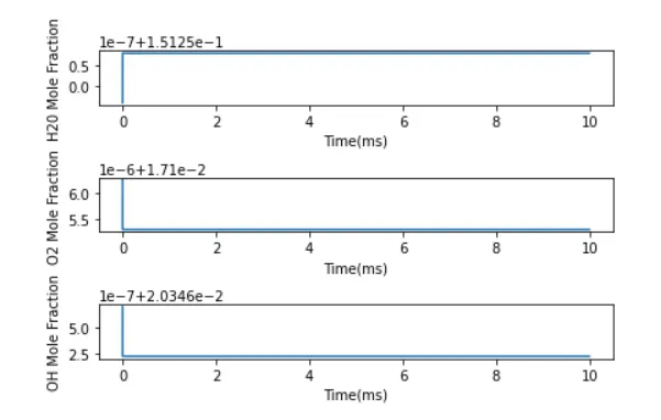
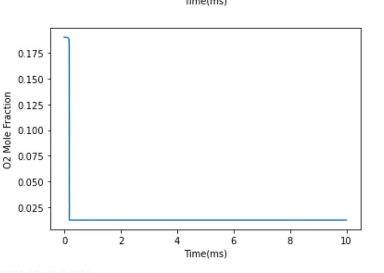
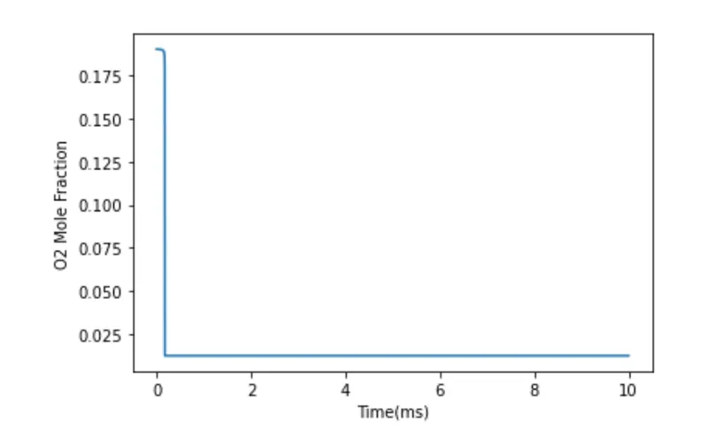
When Temperature is 1000K and pressure 5bar
From the below plots we can infer
- H20 molefraction is less before auto ignition and increases after the ignition
-O2 Concentration decreases because it gets oxidized
-OH molefraction displays a similar trend as H20.
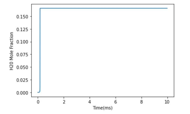
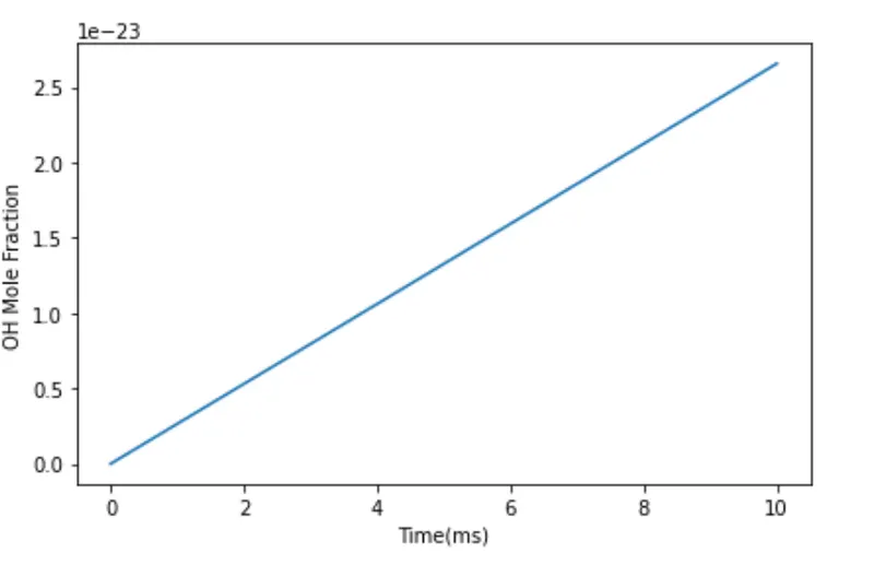
When temperature is 500K and pressure 5 bar
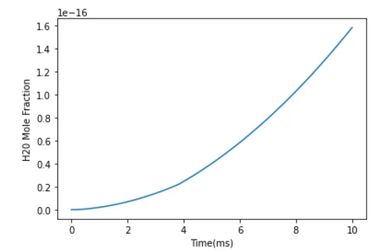
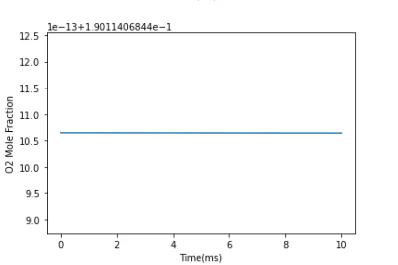
Due to the low temperature it is noted that auto ignition does not takes place. mole fraction of quantities is very less. This signifies the importance of right temperature for auto ignition.
Conclusion
The impact of state properties on auto ignition temperature was examined.