Exhaust Port Challenge

AIM:- The aim of this project is

• Explain where and why a CHT analysis is used
• Maintain the y+ value according to the turbulence model and justify the result.
• Calculate the wall/surface heat transfer coeffiecient on the internal solid surface. Show the velocity and temperature contours in the appropriate areas.
• Verifying whether the HTC predictions fromthe simulations are right. Explaining the factors on which the accuracy of the prediction depends on.

1. CHT ANALYSIS

In a heat transfer between a body and fluid flowing past it, the heat transfer inside the body is governed by Fourier's equation wheras the flow in the fluid is governed by the Navier Stokes equation. The solution to such equation gives the temperature and heat flux distributions on the interface. The conjugate heat transfer is used where a solid and a fluid interacts with each other and we need to know the thermal exchange at the interface within the solids and fluids.

There are many conjugate problems in other fields of science. For instance, studying of subsonic-supersonic flows requires conjugation because the subsonic flow is governed by elliptic or parabolic differential equations, while the supersonic flow is governed by hyperbolic differential equation. Every combustion process has two areas containing fresh and burnt gases with different properties . In biology, diffusion processes usually proceed simultaneously in qualitatively different areas (e.g., in membranes) and, therefore, require a conjugation procedure

2. GEOMETRY

The geometry considered for the analysis is given below

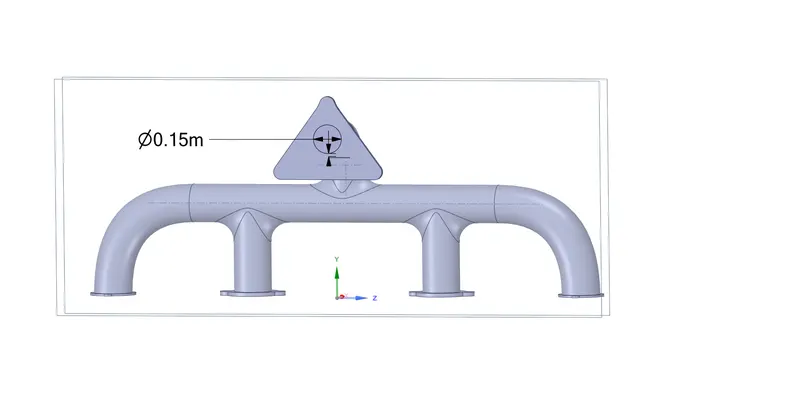
Fig:- Exhaust Port CAD model outlet dimensions

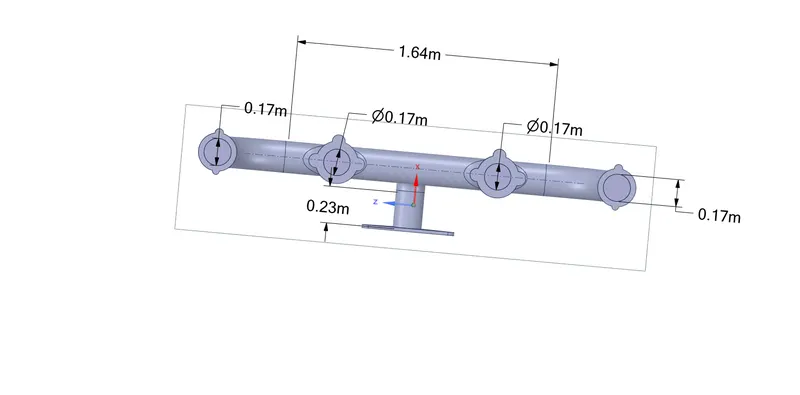
Fig: Geometry Dimensions

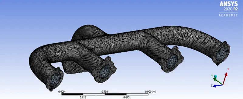
3. MESHING

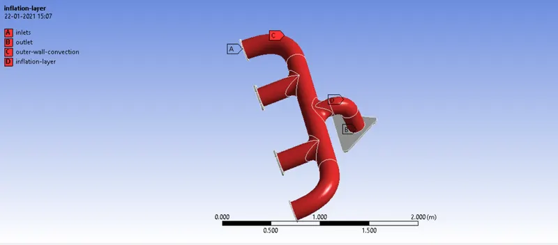
i) Creation of Named Selections

The parts of the geometry were labelled as shown below

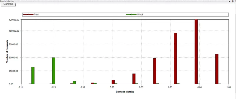
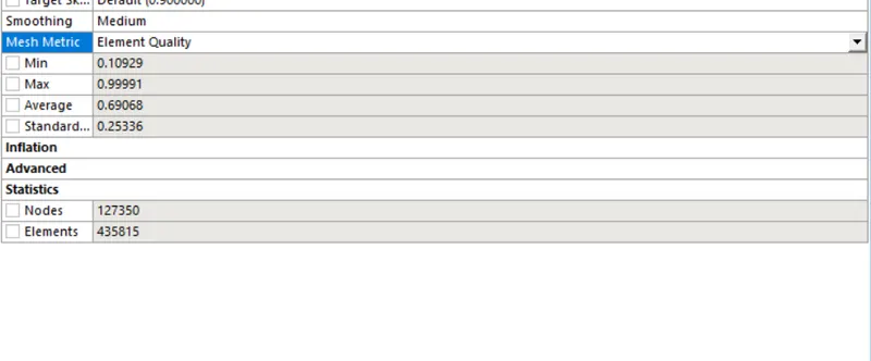
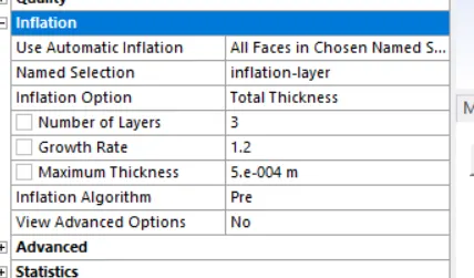
ii) Generation of Mesh

4. Set Up

i) Solver:- Pressure based

Velocity Formulation- Absolute

Time - Steady

ii) Turbulence Model- K omega turbulence model of SST type is used for this analysis. This model is well suited for simulating the flow in the viscous sub layer. This analysis is more pertinent when we want to investigate the near wall conditions and get a more accurate HTC.

iii) FLuid and Solid Material used and its properties

Material	Density	Specific Heat(J/kg-K)	Thermal Conductivity (W/m-K)	Viscosity
Fluid (Air)	1.225	1006.43	0.0242	1.79E-05
Solid (Aluminium)	2719	871	202.4

iv) Boundary Conditions

• The inlet temperature of air is maintained at 700K
• The magnitude of velocity from 4 inlets to the exhaust is 5m/sec
• Outer Wall convection has been assigned a heat transefer coefficient of 20 W/m2-k
• Free stream temperature of 300K
• At outlet pressure has been assumed to be atmospheric pressure and gauge pressure is maintianed at 0 Pa.

5. Results

i) Residuals

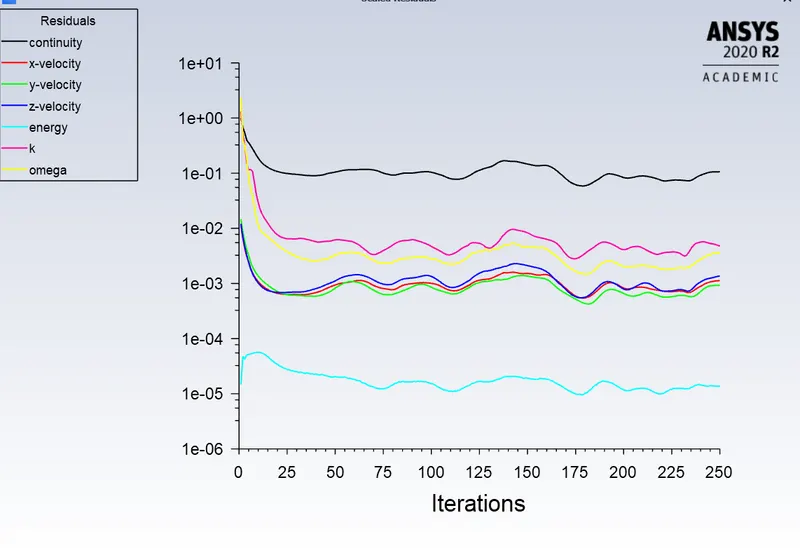
Fig:- The above shows convergence of various k-omega parameters.

ii) Heat Transfer Coefficient Analysis

• At Plane 1

A Plane was created on the pipe that connects inlets to exhaust as shown below

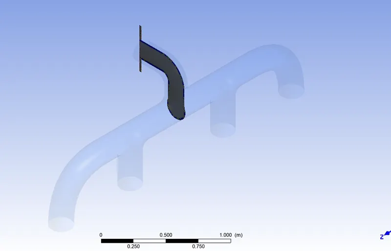
The Heat transfer coefficient was plotted on this plane and is given below.

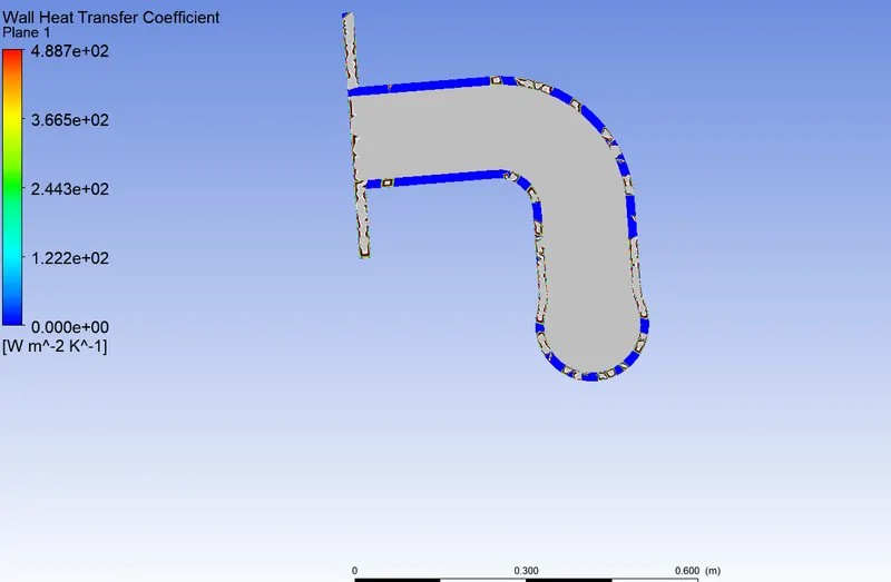
Using Function calculator the Maximum, average and mean values were computed

Plane 1	HTC [W m^-2 K^-1]
Average	104
Maximum	483.928
Minimum	0

iii) Temperature Contour Analysis at Plane 1

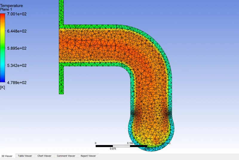
From the above plot it is inferred that the maximum temperature of the fluid occurs in the internal region. THe maximum value is computed to be 690.635K. This occurs in the central region of the plane. As we move closer to the wall the temperature displays a decreasing trend reaching a minimum value of 526.588K. THis is due to the existence of a temperature gradient between fluid and solid regions, fuild containing the hot exhaust gases much higher than the solid ambient.

iv) Velocity contour Analysis

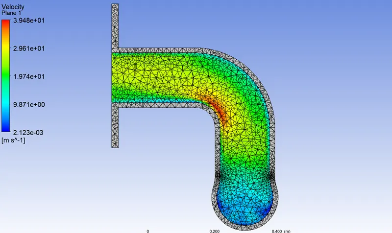
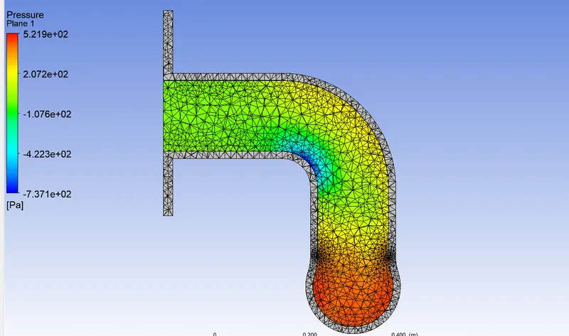
The maximum value of velocity is calculated to be 42.1m/s and it occurs at the inner elbow of the geometry. Fluid entering the exhaust at an average velocity of 20m/s, when subjected to a change in direction loses pressure.This loss in pressure manifests itself to an increased fluid velocity. This is the probable region for increased velocity in the inner radius od the bend. The minimum value is computed to be 0.294666 [m s^-1] and it occurs near the outlet.

It is to be noted that the velocity in this plane is significantly higher than the inlet velocity of 5m/s in each of the inlet port. THis can be explained by using mass conservation. The outlet from five inlet ports of similar when combined to a common exhaust port of reduced area results in increased velocity.

v) Calculation of Y+ value Theoretically

Y+=(rho*Y*V)/('mu')

Y=0.000005 m

rho= 1.225 kg/m^3

'mu'= 2*10^-5 kg/m-sec

Y+ is calculated to be 3 which is equal to what was considered.

vi) Verification of Heat Transfer coefficient (Plane 1)

Q= h*A*delta T

vii) Maximum heat flux and Area of the plane are determined from function calulator

Q=15000

A= 0.146417 [m^2]

delta t = 223 k

h is calculated to be 460 W/m2 K which is close to the value obtained from ANsys fluent (483.33)

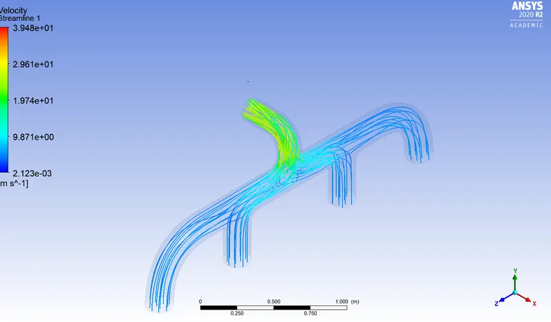
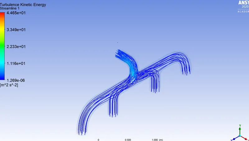
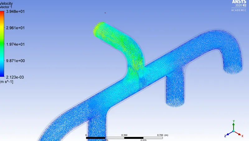
viii) Streamlines and path lines for Velocity and KE

Conclusion

In this problem the CHT phenomenon was analysed using k - omega turbulence model

1) The wall heat transfer coefficient was computed from ansys fluent and the same was verified using theoretical calculation.

2) THe y+ value was calculated theoretically and the number of inflation layers were found to be in agreement with what was considered

3) The heat transfer coefficent depends upon the thermal properties of a medium, the hydrodynamic characteristics of its flow, and the hydrodynamic and thermal boundary conditions. SOme of these factors are listed below.

• Fluid-solid combination
• Geometry of the solid surface
• Temperature range of fluid and solid
• Convective velocity of the fluid phase