FLOW THROUGH A FLOW BENCH.

1. Objective:-

i. Create a 3D model of a flow bench and run flow analysis. obtaining a plot of lift vs mass flow rate.
ii. Grid dependence test For three grids run your simulation at a particular valve lift and explain your results.
iii. Effect of valve lift on the mass flow rate.
iv. Once you have decided the best grid, run a parametric sweep to show the effect of valve lift on the mass flow rate.

2. Basic:-

A flow bench is a device used for testing the internal aerodynamic qualities of an engine component and it is related to the more familiar wind tunnel. It is used primarily for testing the intake and exhaust ports of cylinder heads of internal combustion engines. It is also used to test the flow capabilities of any component such as air filters, carburettors, manifolds or any other part that is required to flow gas. A flow bench is one of the primary tools of high-performance engine builders, and porting cylinder heads would be strictly hit or miss without it.
A flow bench consists of an air pump of some sort, a metering element, pressure and temperature measuring instruments such as manometers, and various controls. The test piece is attached in series with the pump and measuring element and air is pumped through the whole system. Therefore, all the air passing through the metering element also passes through the test piece. Because the volume flow rate through the metering element is known and the flow through the test piece is the same, it is also known. The mass flow rate can be calculated using the known pressure and temperature data to calculate air densities and multiplying by the volume flow rate.
Here we are taking the only intake port not an exhaust port because the flow bench uses only those ports which will be going to test.

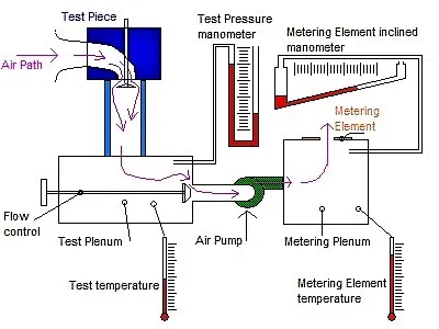
Grid dependence test:- The Grid dependence test is also known as the Mesh dependency test in which simulating the same body at a refined mesh size. The grid dependency test plays an important role in the simulation. As the mesh size refines the accuracy of the result is getting high hence it is important to select the proper mesh size to minimize error.

3. Procedure:-

Step-1: Creating the 3D model of a flow bench as shown below.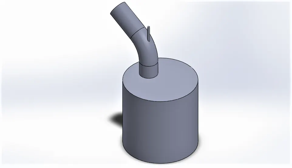

Step-2: Opening the flow simulation add-in for setting up the simulation parameters. i.e. taking flow type as internal flow and fluid type as air and other parameters.

Step-3: Defining the boundary condition such as Total pressure at the inlet and static pressure at outlet and mass flow rate at the inlet.

Step-4: Setting mesh size and doing Grid dependence test for the best mesh size.

Step-5: Setting parametric study for variable valve lift. We are taking valve lift Variation from 0.001 m to 0.008 m and the number of values is 7. Also setting the input and output variable.

Step-6: Run the calculation.

4. Simulation and Analysis:-

Before analysis, we need to do grid Dependency test to get the appropriate mesh size.

4.1 Grid Dependency Test:- In the grid dependency test, we are going to use the valve lift of 0.004500m for and the mesh size of 3,4 and 5 respectively.

Simulation Parameters:

Unit	: SI
Static Pressure	:101325 pa
Total Pressure	: 501325 pa
Mass flow rate	: 1 m/s

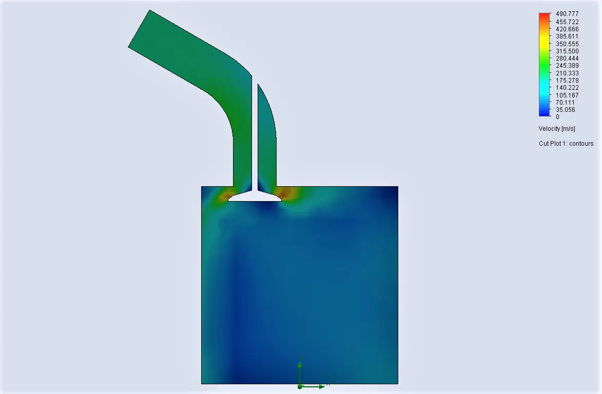
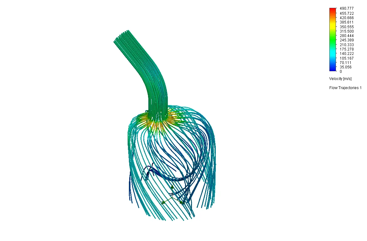
i. At Refinement level-3:

Cut plot:

Flow Trajectories:

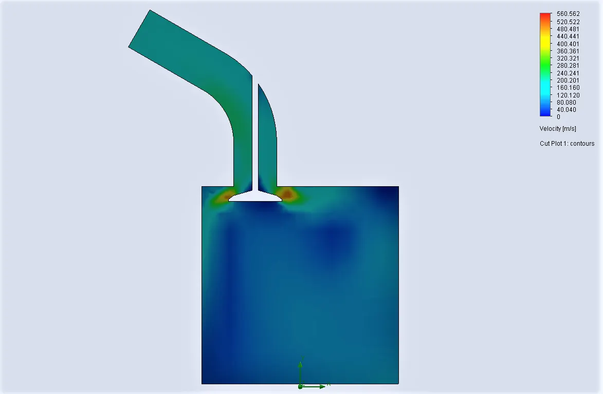
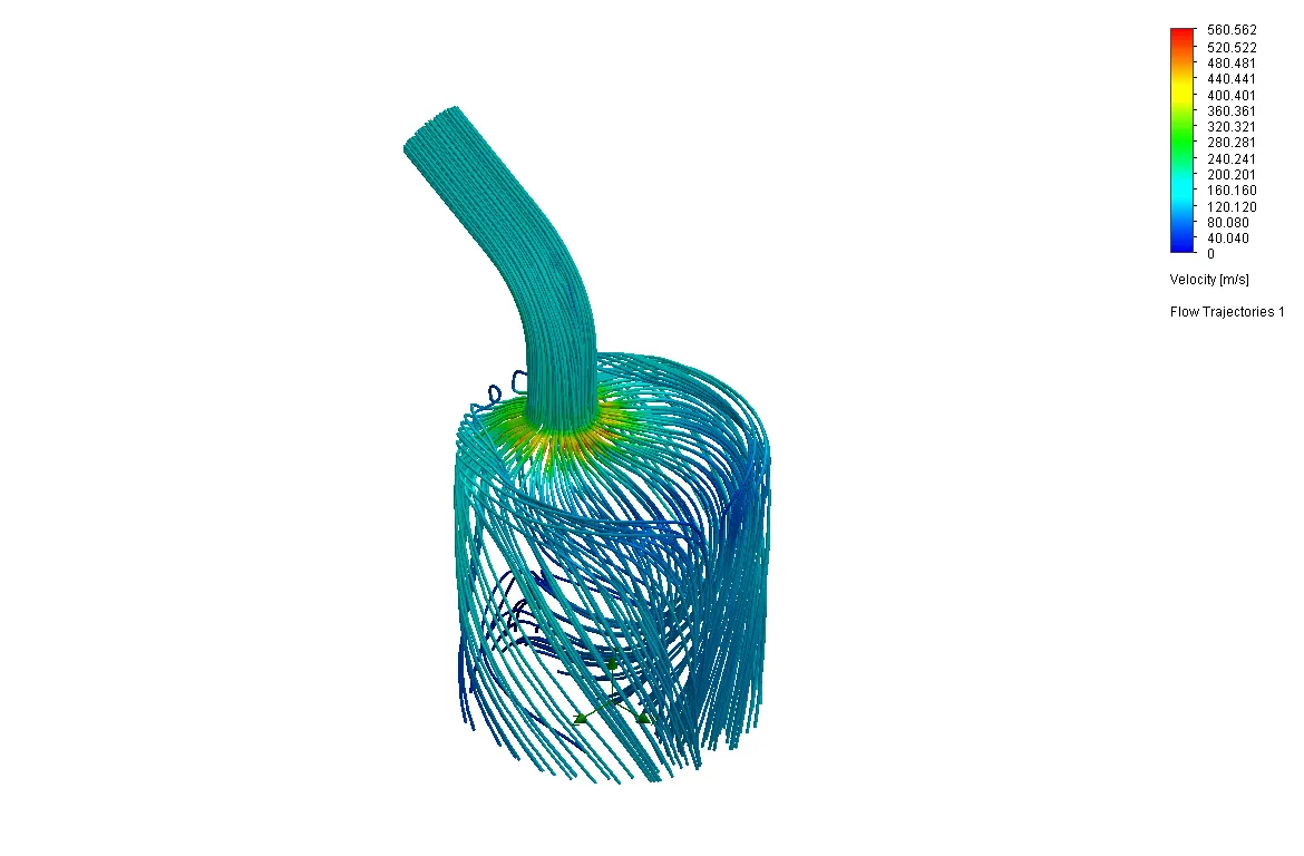
ii. At Refinement level-4:

Cut plot:

Flow Trajectories:

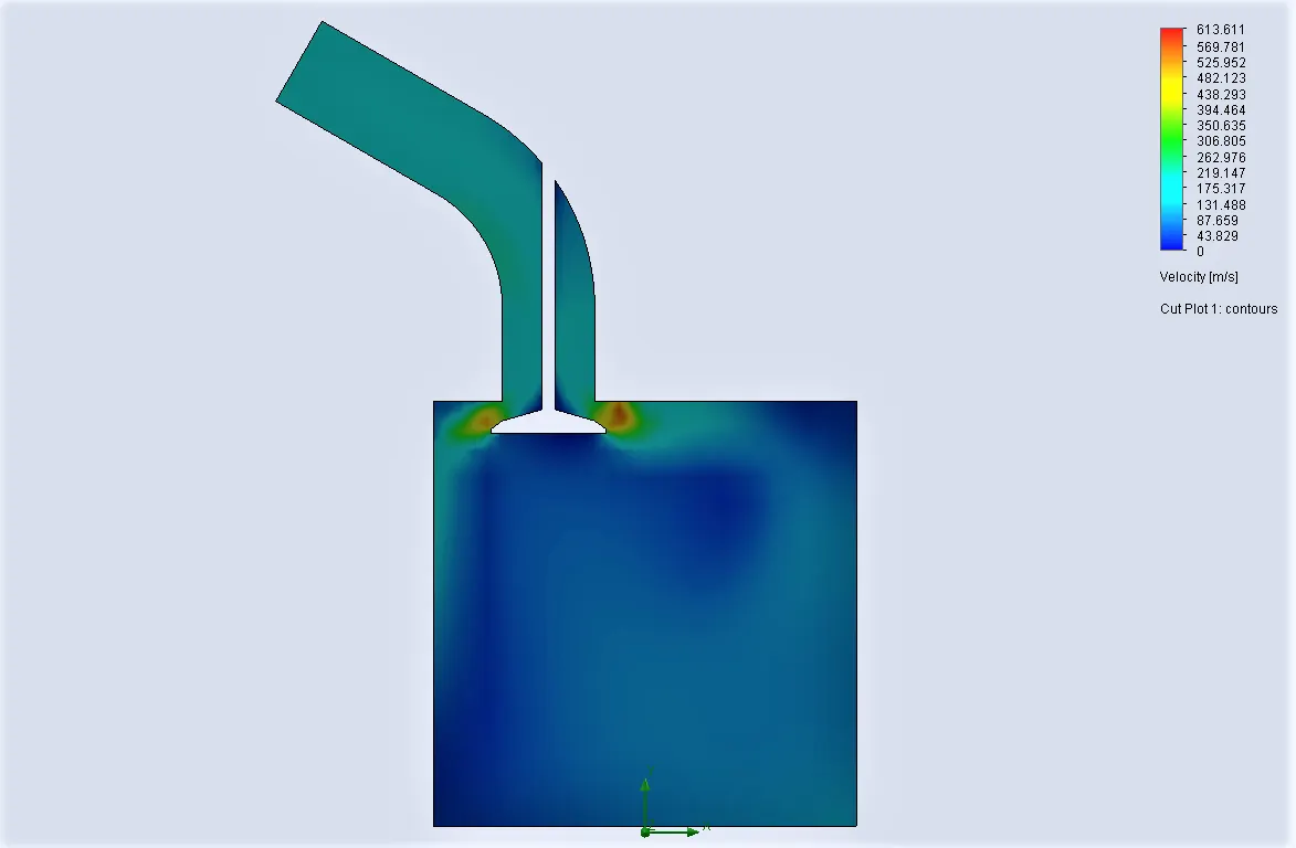
iii. At Refinement level-5:

Cut plot:

Flow Trajectories:

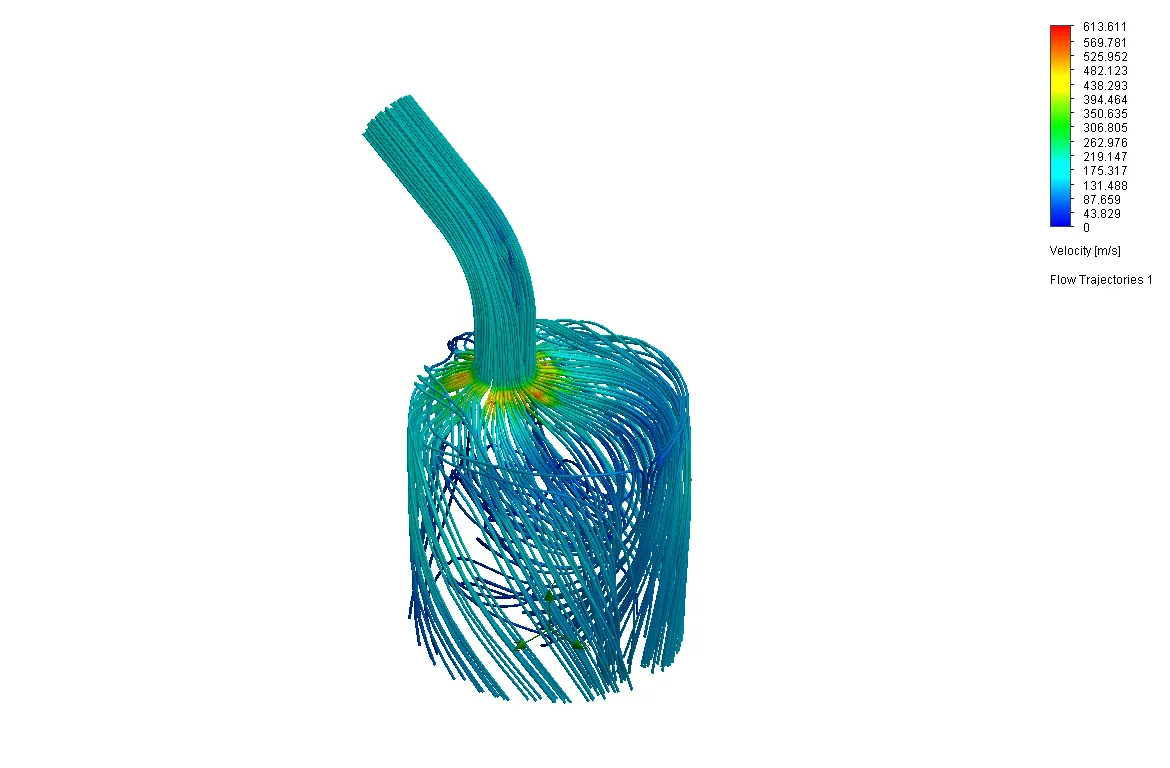
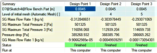
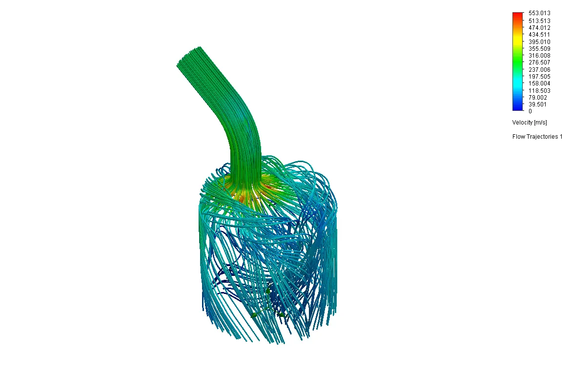
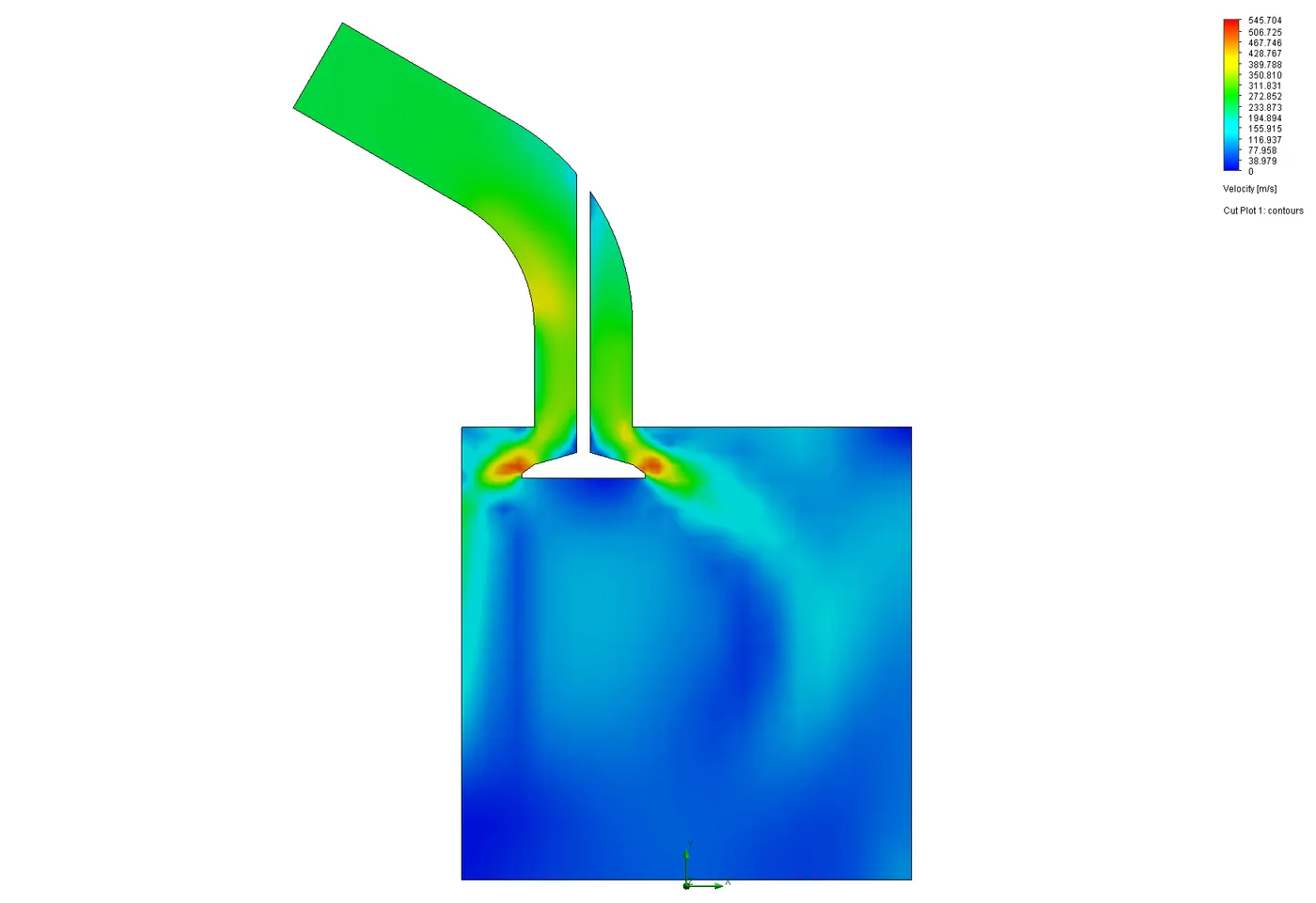
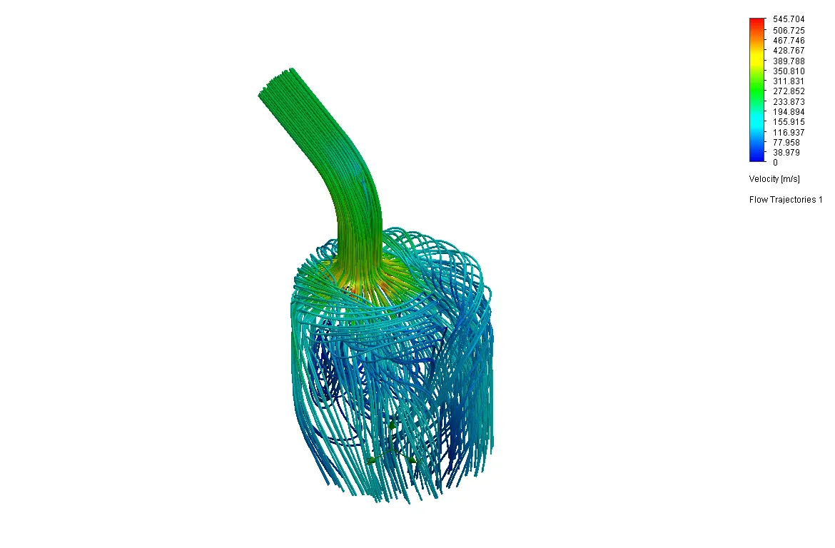
from the grid dependency test, we can see that the mesh size 5 is giving more clear result and also the flow trajectories is visualized more clear. Hence in further studies, we will use the mesh refinement level to 5.

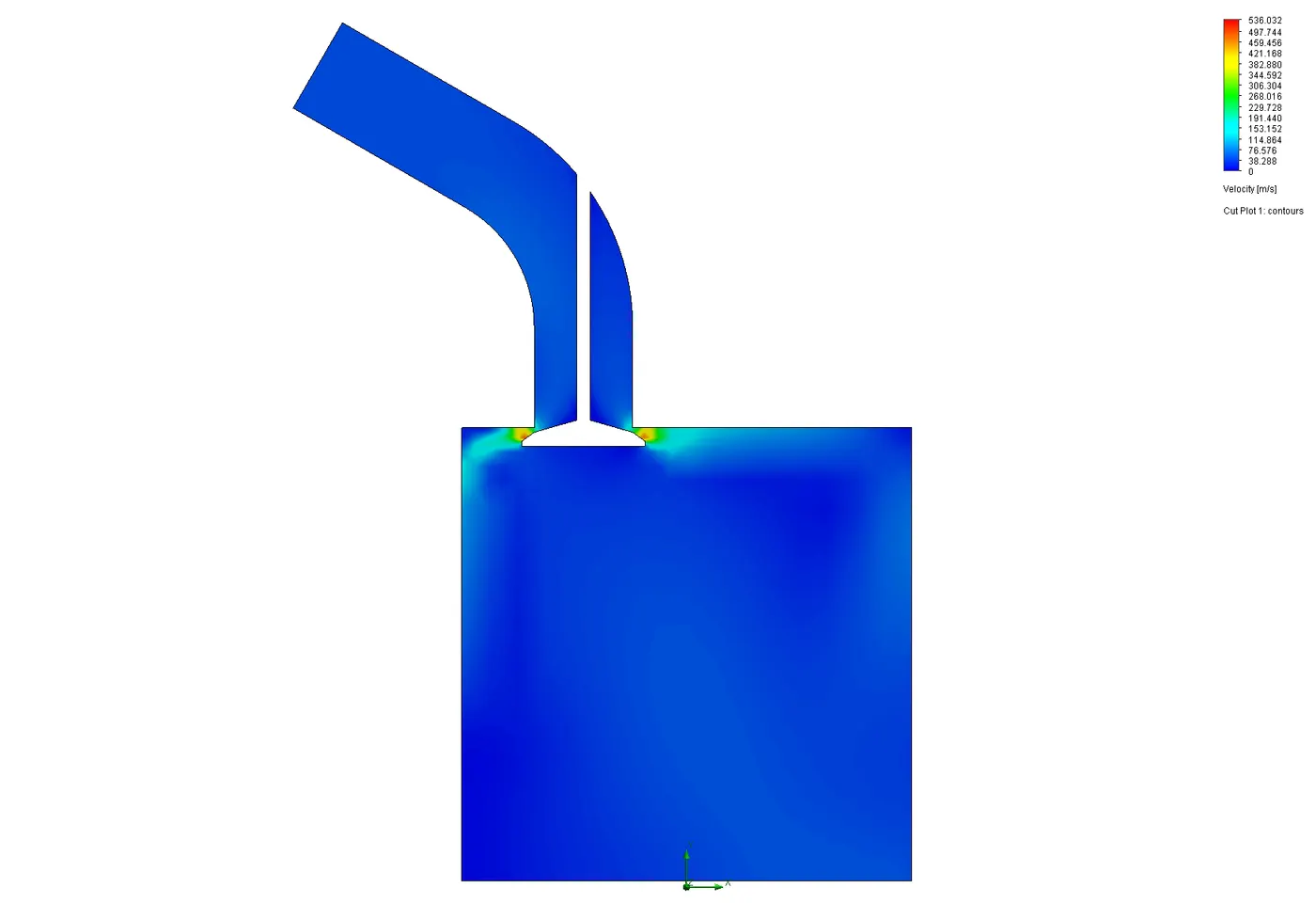
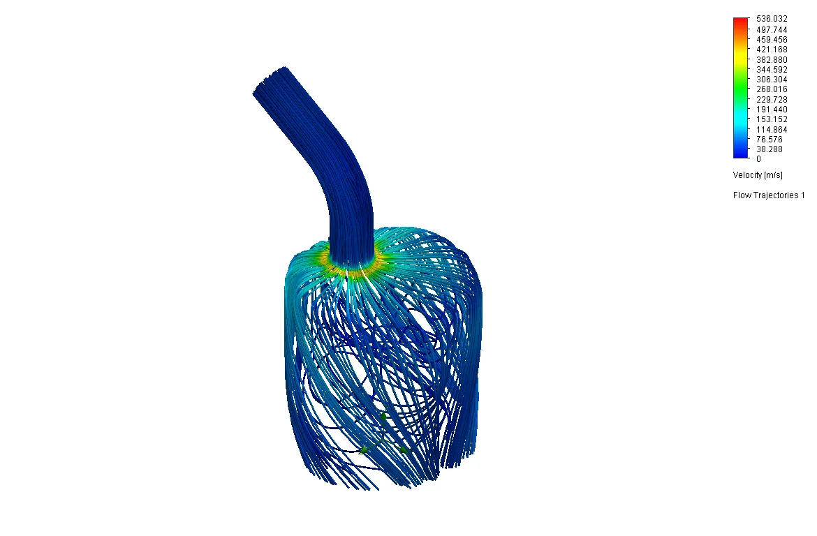
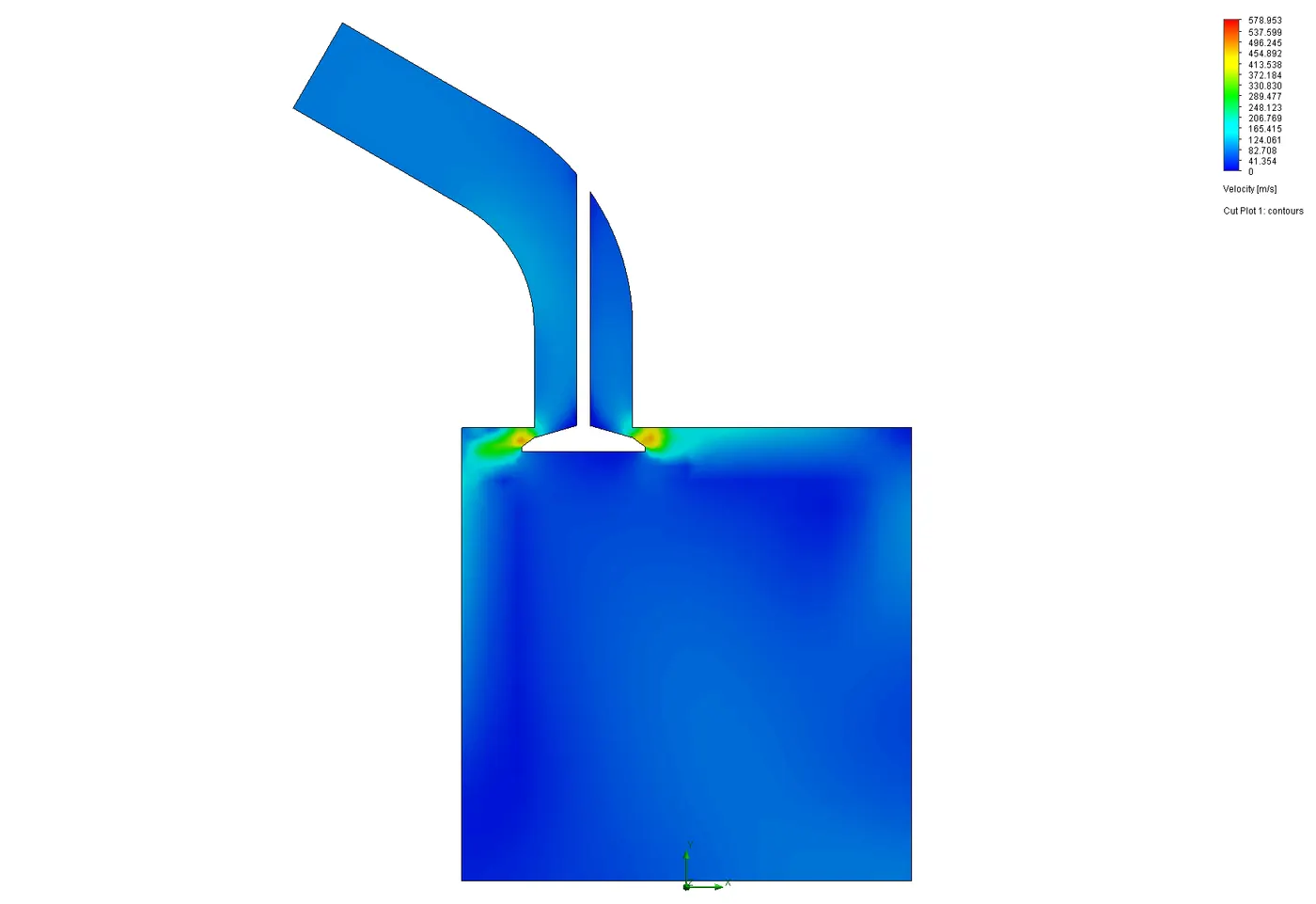
4.2 Cases of Valve Lift:- We are taking valve lift Variation from 0.001 m to 0.008 m and the number of values is 7. In this the mesh size of the 5 for better result. In each valve lift, we are taken the cut plot and the flow trajectories to represent the flow behaviour.

i. At valve lift 0.001m:-

Cut plot:

Flow Trajectories:

ii. At valve lift 0.0021667m:-

Cut plot:

Flow Trajectories:

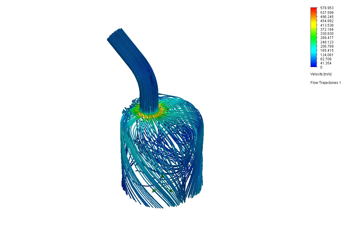
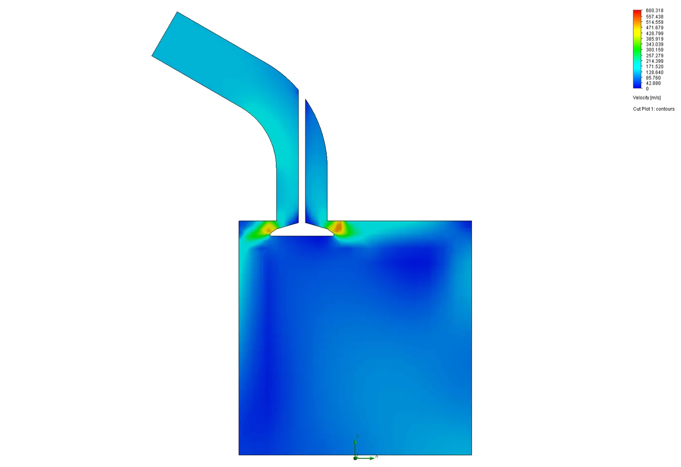
iii. At valve lift 0.003333m:-

Cut plot:

Flow Trajectories:

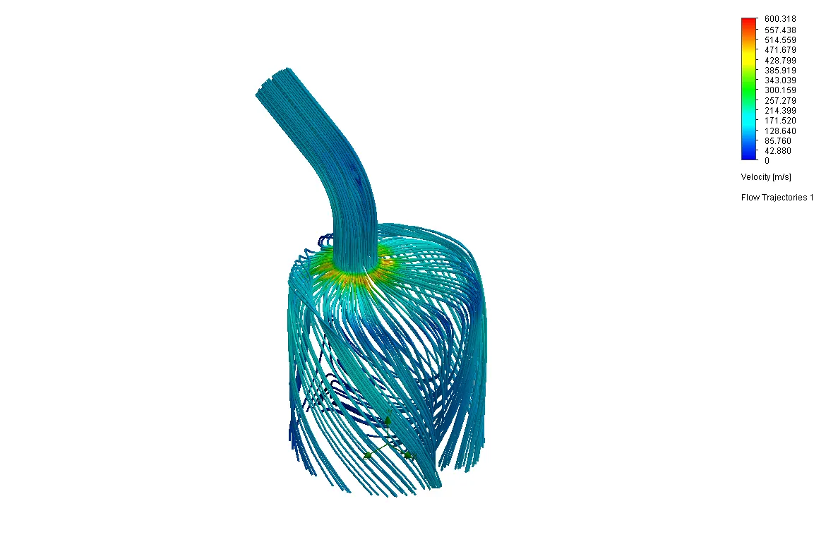
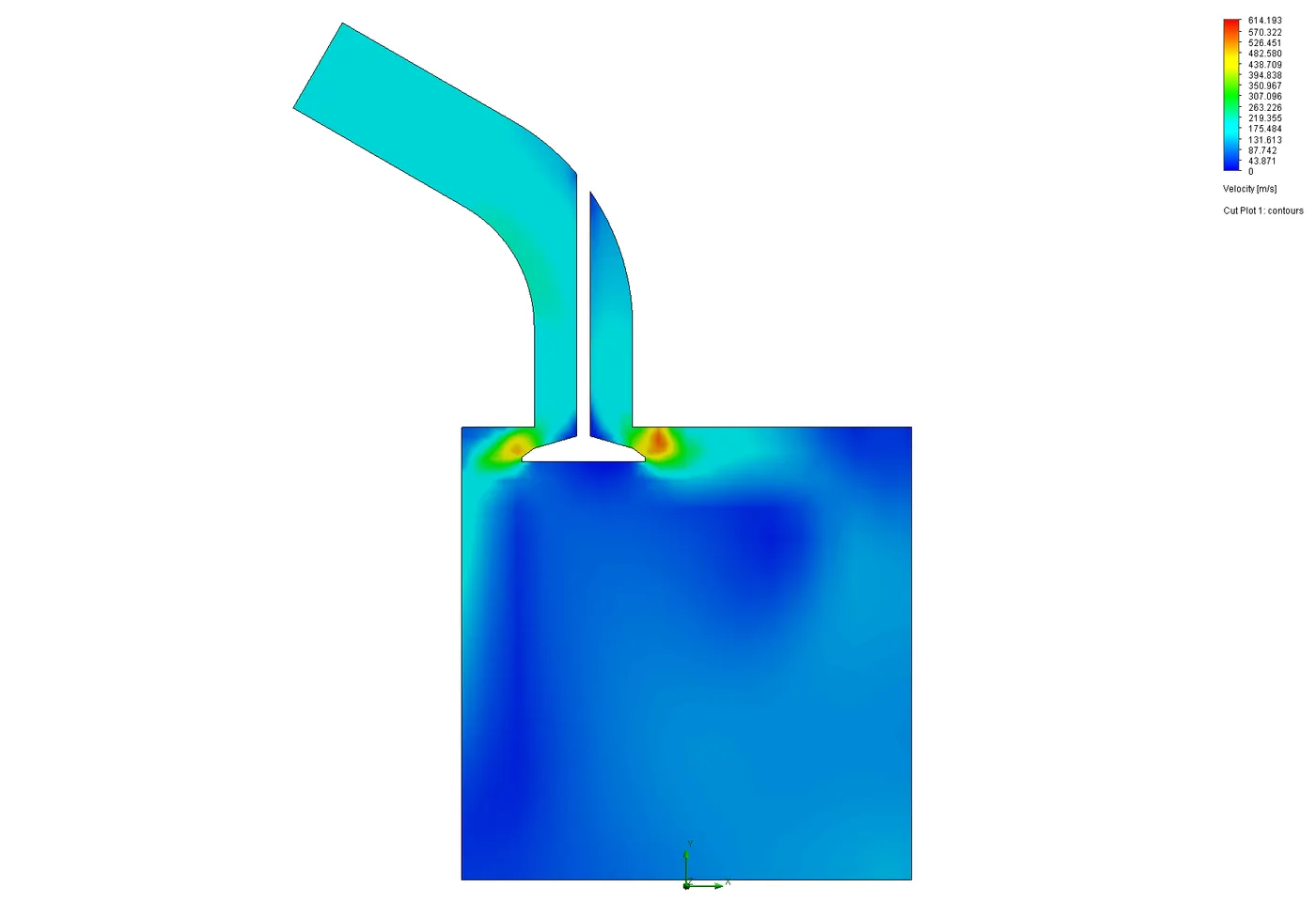
iv. At valve lift 0.004500m:-

Cut plot:

Flow Trajectories:

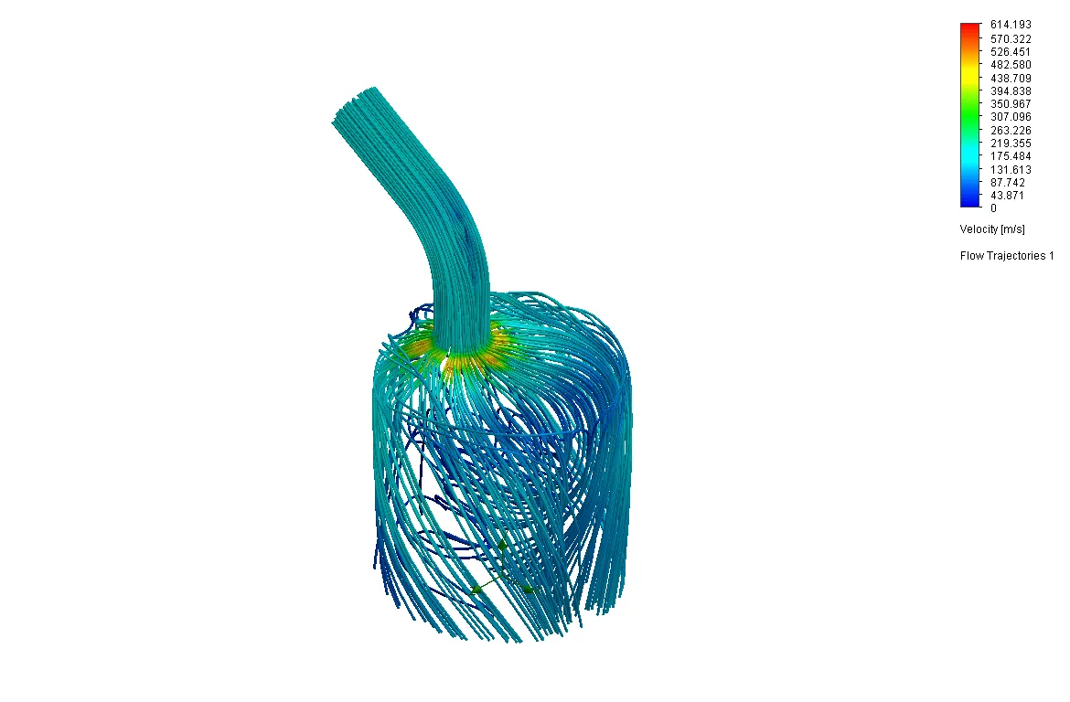
v. At valve lift 0.005666m:-

Cut plot:

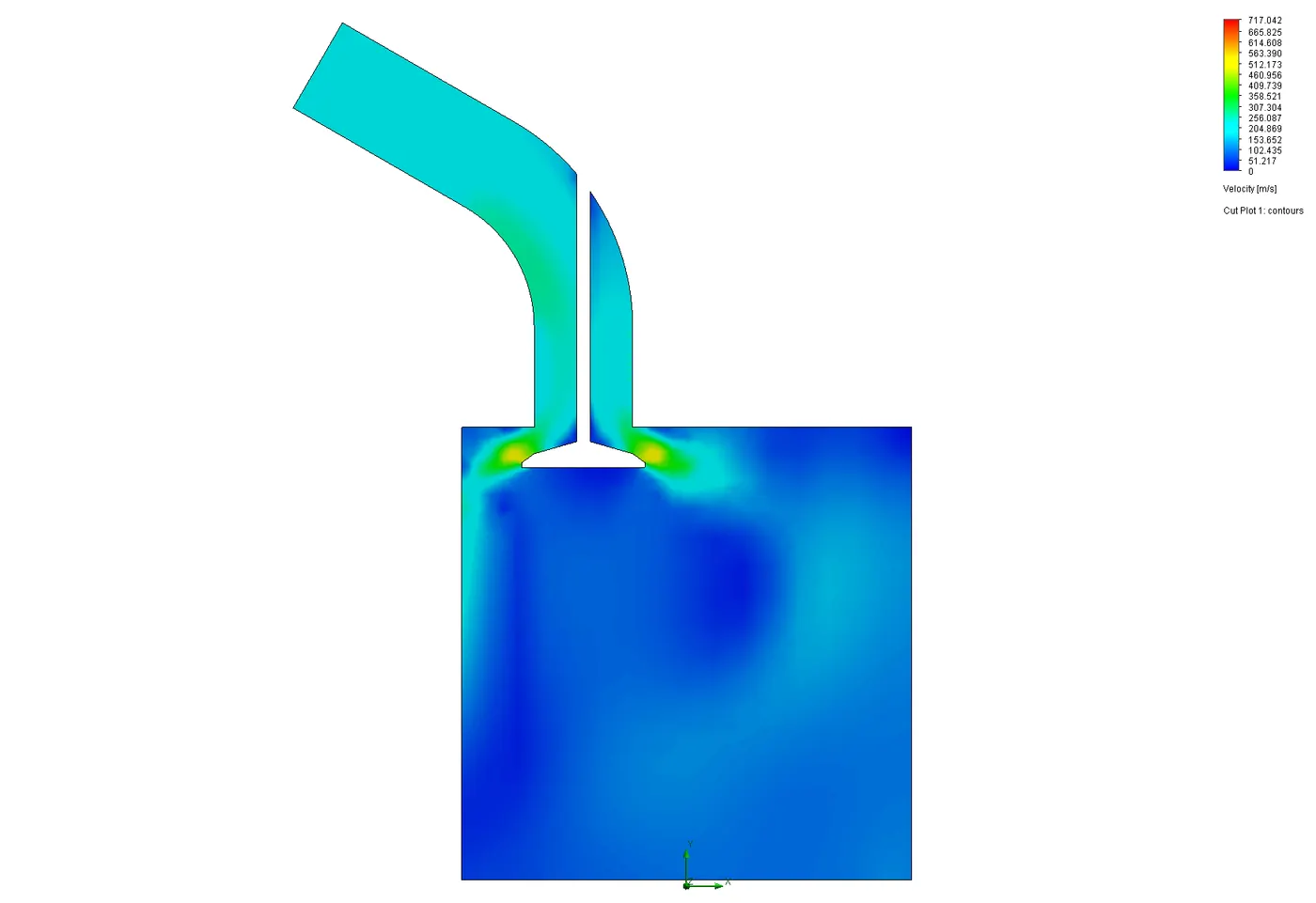
Flow Trajectories:

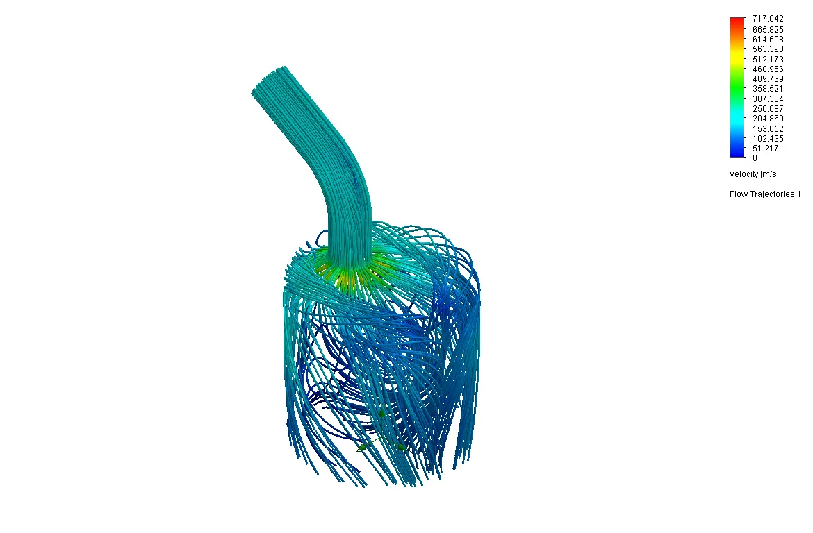
vi. At valve lift 0.006833m:-

Cut plot:

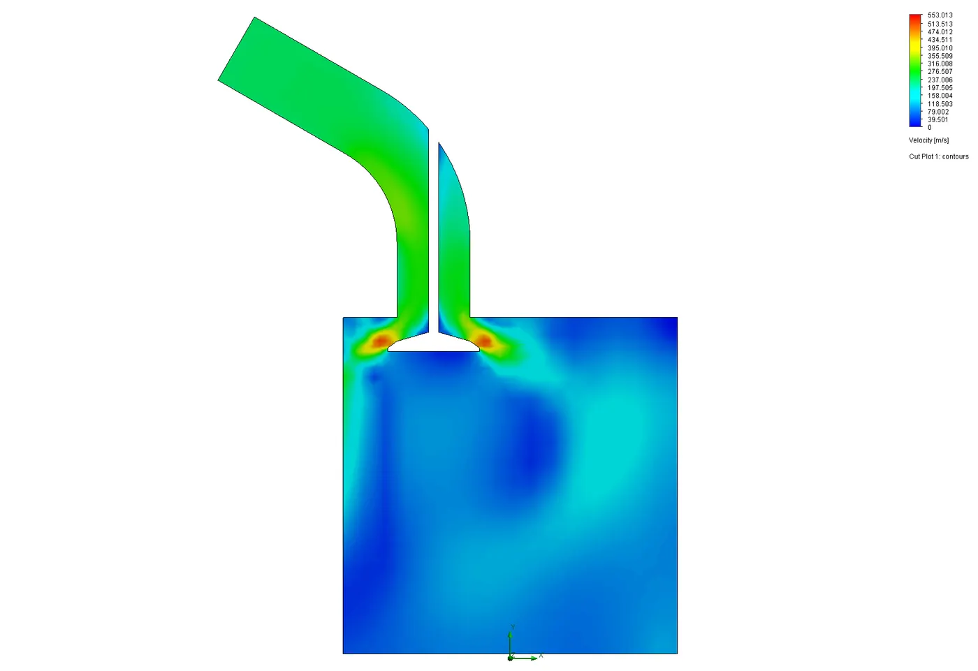
Flow Trajectories:

vii. At valve lift 0.008m:-

Cut plot:

Flow Trajectories:

5. Observation and Conclusion:-

From the above simulation and analysis studies, we can conclude the major three result as follows.

5.1 Mass Flow Rate (vs) Valve lift:-

Mass Flow Rate 1 [kg/s] at Design points is as follows.

Design Point 1	Design Point 2	Design Point 3	Design Point 4	Design Point 5	Design Point 6	Design Point 7
-0.095927299	-0.166328182	-0.23742248	-0.292934601	-0.331863903	-0.351788883	-0.357704277

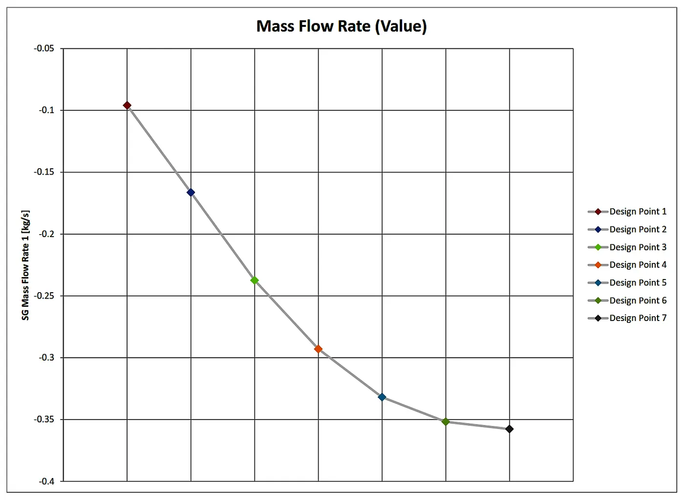
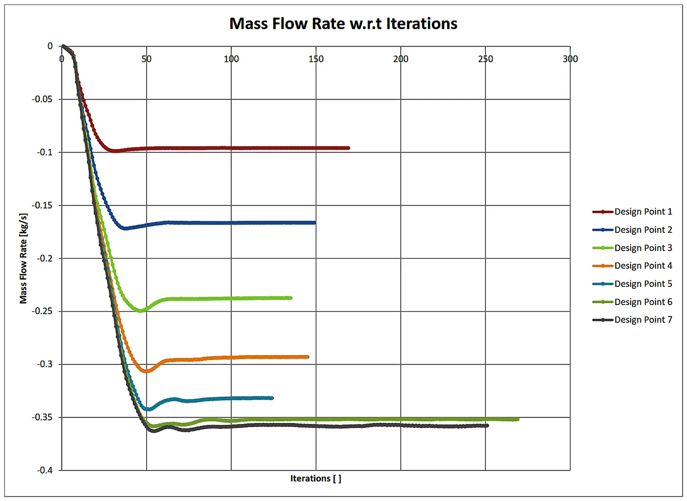
From the plot of the mass flow rate with respect to the valve lift, we can see that plot having a negative value which represents that flow leaving from the system. hence as the valve lift increases the mass flow rate increases but represented by the negative value as discussed.
Also, as the mass flow rate increases with respect to the valve lift the variation is seen in the above first plot is linear. The variation is linear initially up to the certain value after that it increases but variation in the curve is seen smaller and the value of the mass flow rate is also smaller.
This is caused due to the reverse force applied (based on newton's 3rd law) by the valve on the flowing fluid in the system. This reverse force is higher in the initial stage and it decreases with increasing the valve lift and makes the curve path in the plot.

5.2 Pressure Drop:-

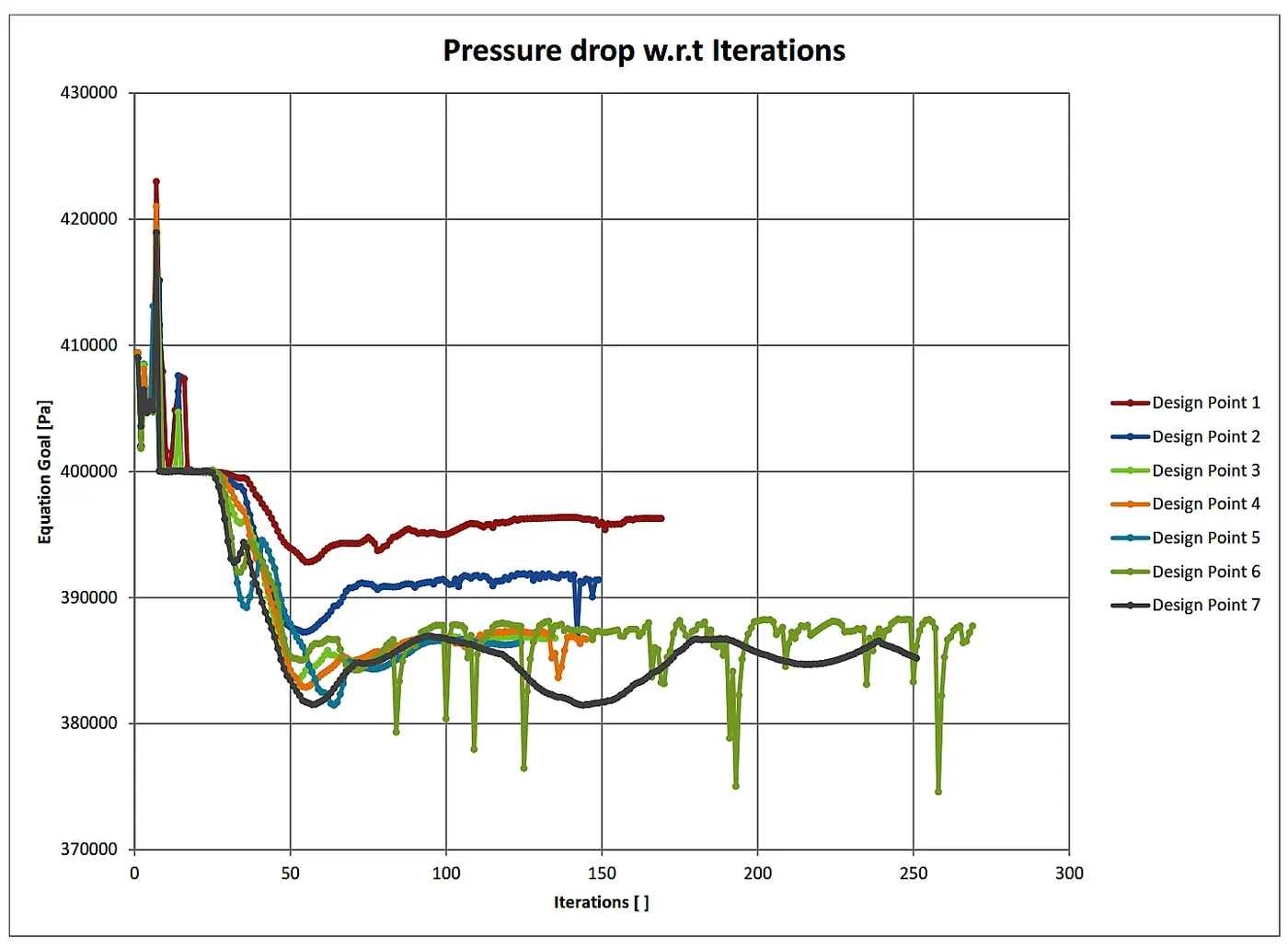
5.2.1 Pressure drop at design points: The pressure drop at a design point can be calculated with the formula is given below as,

"Pressure Drop = Maximum Total Pressure at the inlet - Maximum Total Pressure at the Outlet"

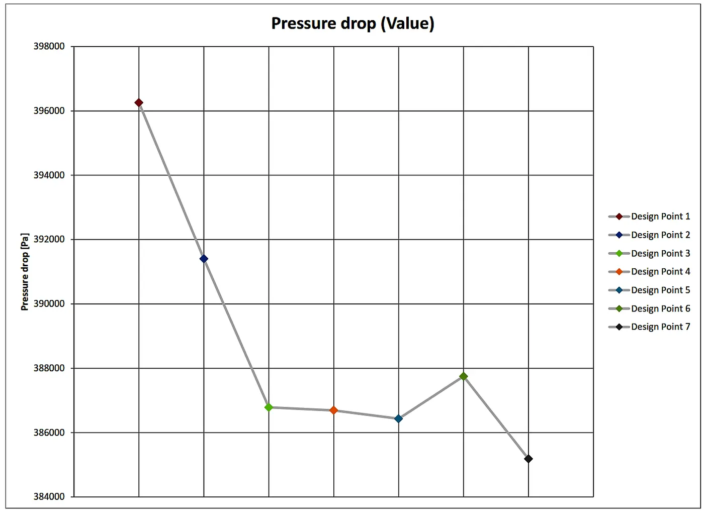
Hence the calculated Pressure Drop at Design points (Pa) is as follows.

Design Point 1	Design Point 2	Design Point 3	Design Point 4	Design Point 5	Design Point 6	Design Point 7
396256.8888	391402.8527	386784.7056	386691.9285	386430.9888	387748.0175	385180.1489

5.2.2 Overall Pressure Drop:- The overall pressure drop with respect to the valve lift can be calculated from the formula as follows.

"OPD = pressure Maximum Pressure at the Design point 1 - Maximum Pressure at the Design point 7"

396256.8888 - 385180.1489 (pa)

(or)

396.2568888 - 385.1801489 (kpa)

OPD = 11,076.7399‬ pa (or) 11.0767399 kpa

From the above results, we can conclude that as the valve lift increases the pressure drop is decreases but the overall pressure drop from the design point 1 (i.e at valve lift 0.001m) to the design point-7 (i.e at valve lift 0.008m) is 11.0767399 kpa which is minimum. Hence for the flow bench, the pressure drop should be minimum.

5.3 Flow Behavior To changes in Valve Geometry:- The flow behaviour changes in the valve geometry can be represented from the animation of the cut plot and flow trajectories as shown below.

In each valve lift, the cut plot animation to represent the flow behaviour.

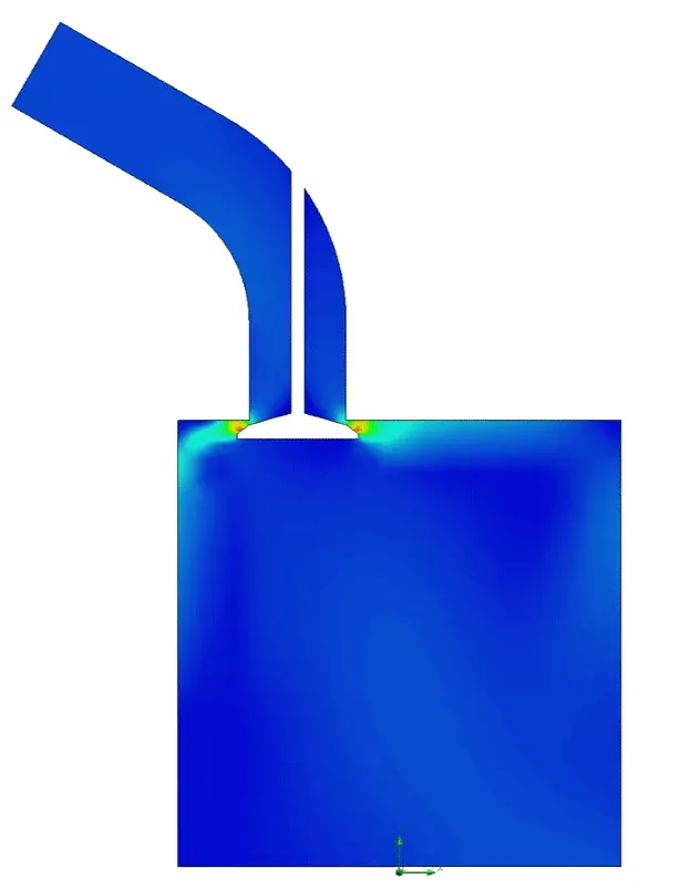
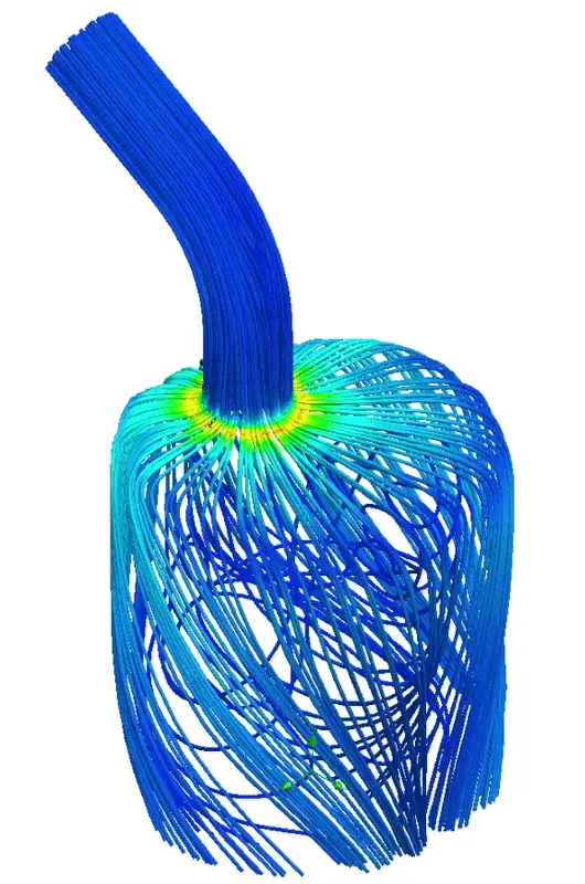
In each valve lift, the flow trajectories animation to represent the flow behaviour. In the above Animation of the cut plot and flow trajectories with respect to the valve lift, the blue region indicates a minimum velocity at a point on the surface of the valve while the red region indicated that the maximum velocity. Also in the inlet port, the colour changing from the blue to the green as the valve is lifted indicates an increase in velocity.

Reference:-

https://en.wikipedia.org/wiki/Air_flow_bench
https://www.youtube.com/watch?v=l04OPFeqfPY&t=100s

The flow of report:-

1. Objective.

2. Basic.

3. Procedure.

4. Simulation and Analysis.

5. Result and conclusion.