FLOW OVER A CYLINDER.
1. Objective:-
i. To Run a baseline simulation and calculate the Reynolds number.
ii. Increase the Reynolds number by a factor of 20%, 40%, and 100% then run the transient flow simulation.
iii. Create animations for pressure-velocity for all the three Reynolds numbers.
2. Concepts:-
Before simulation we need to understand some basic terms related to the fluid flow over the body. the basic terms are as follows.
2.1 Basic Terms:-
i. Separation point and Wake Region: The position at which the boundary layer leaves the surface of a solid body. It may occur with the laminar flow (laminar separation) or when the boundary layer is turbulent (turbulent separation). Separation is sometimes followed by reattachment of the flow.
The thickness of this layer is smallest at the stagnation point and increases towards the backside of the obstacle. However, at some point on the backside, the boundary layer separates from the obstacle's surface to form a vortex-filled wake whose transverse dimensions are similar to those of the obstacle itself. This phenomenon is known as boundary layer separation.
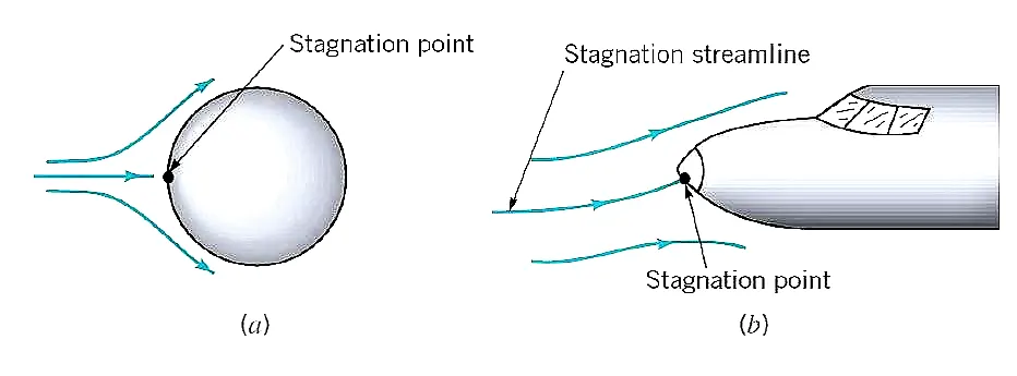
ii. Stagnation point: In fluid dynamics, a stagnation point is a point in a flow field where the local velocity of the fluid is Minimum (or) zero and static pressure acting on the body is maximum. Stagnation points exist at the surface of objects in the flow field, where the fluid is brought to rest by the object.
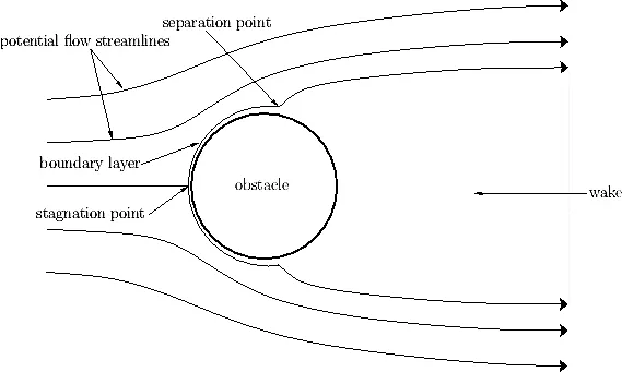
the flow separates from the surface and creating a highly turbulent region behind the cylinder called the wake.
iii. Vortex Shedding: The boundary layer separates from the surface forms a free shear layer and is highly unstable. This shear layer will eventually roll into a discrete vortex and detach from the surface (a phenomenon called vortex shedding). Another type of flow instability emerges as the shear layer vortices shed from both the top and bottom surfaces interact with one another. They shed alternatively from the cylinder and generates a regular vortex pattern (the Karaman vortex street) in the wake. The vortex shedding occurs at a discrete frequency and is a function of the Reynolds number. The dimensionless frequency of the vortex shedding, the shedding Strouhal number, St = f D/V, is approximately equal to 0.21 when the Reynolds number is greater than 1,000.
2.2 Equations:
The type of flow is decided based on Reynold's number which is based on the density of fluid, Velocity of fluid, diameter, and viscosity.
`[Re = (ρ*V*D)/μ]` .................(i)
Where:-
ρ = Density
V = Velocity
D = Diameter of pipe
μ = Viscosity
In our Problem, we need the help of Reynold's number and increase it to the factor of 20%, 40%, and 100% and do simulation according to it. After that, We need to calculate the time duration for flow-through time. the time calculation based on the following formula.
`[Time=(Distance)/(Velocity)]` .................(ii)
Where:-
Time = flow-through time;
Distance = Length of the computational domain;
Velocity = calculated velocity for each case.
Other than These we need to understand some other basic terminology which is as follows.
2.3 Basic Terminology:
i. Computational Domain and its Dimensions:
The computational Doman is the simplified form of a physical domain which is sufficient to consider the geometry in the simulation and also to impose the boundary conditions
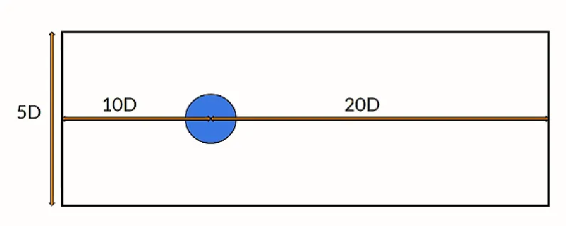
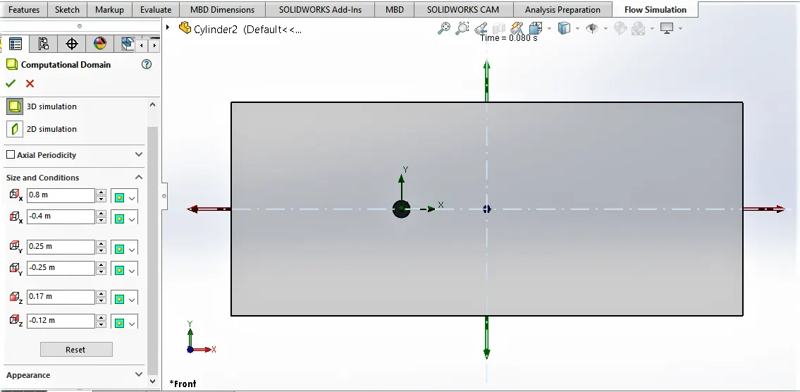
this simplified form should retain all physically important features of the problem. considering this as the environment to the system the boundary condition is provided accordingly. here the geometry is cylindrical. also, the basic dimension provided for the computational domain is as shown below.
ii. Transient Simulation: transient simulation is where the time derivative of the variable are also taken into account, hence the magnitude of the values of the system can be monitored at any particular instant of time but in steady-state simulation, only the initial values and steady-state values can be obtained.
In this project, we are approaching the solution through a transient simulation in order to observe the flow variables at each and every timestep. this will also help us in monitoring the frequency of the vortex shedding with respect to various Reynolds numbers.
iii. Total Analysis time(TAT):- The total analysis time defines the physical time period until which the simulation will be run from its initial instant of time.
iv. Flow-through time(FTT):-The time required for the flow to pass through the domain.
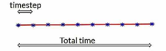
v. Output time steps(OTS):- Time step is used in transient solving which denotes the time interval for which the simulation will progress between each iteration/step. in our simulation the time step is 10 for each case.
3. Calculations:-
In All the Cases of simulation, we took the Diameter of the cylinder as 0.04m and length of the cylinder 0.05m. Also, the working fluid is air with density 1.225Kg/m^3 and viscosity as 18*10^-6 N.sec/m^2.
3.1 Baseline:
In the baseline simulation, we took the Velocity as 10m/s and doing the simulation with the total analysis time with 0.1sec and output time step 0.01sec. The calculation of the Reynolds number is as follows.
Reynold's number calculation:
from equation (i)
`Re= (1.225*10*0.04)/(18*10^-6)`
`Re=27222.22`
After calculating Reynold's number for the baseline we need to increase it with a factor of 20%, 40%, and 100% and calculating the velocity and effective time duration for the simulation as follows.
3.2 Increasing (Re) factor of 20 Percentage:
Increasing the Re:
`Re=1.20*27222.22`
`Re=32666.66`
Velocity calculation:
From Equation (i)
`32666.66= (1.225*V*0.04)/(18*10^-6)`
`V=11.999` m/s
Time calculation:
from equation (ii)
`T=11.999/0.8`
`T=0.067` sec
`OTS=0.0067` sec
Similarly, We can calculate other Parameters for the remaining cases.
3.3 Increasing (Re) factor of 40 Percentage:
Increasing the Re:
`Re=1.40*27222.22`
`Re=38111.11`
Velocity calculation:
`38111.11= (1.225*V*0.04)/(18*10^-6)`
`V=13.999` m/s
Time calculation:
`T=13.999/0.8`
`T=0.0571` sec
`OTS=0.00571` sec
3.4 Increasing (Re) factor of 100 Percentage:
Increasing the Re:
`Re=2*27222.22`
`Re=54444.44`
Velocity calculation:
`54444.44= (1.225*V*0.04)/(18*10^-6)`
`V=19.999` m/s
Time calculation:
`T=19.999/0.8`
`T=0.0400` sec
`OTS=0.00400` sec
Final Parameters Table:
| Type | Reynold's Number | Velocity(m/s) | FTT(sec) | TAT(sec) | OTS(sec) |
| Baseline | 27222.22 | 10.000 | |||
| 20% Factor | 32666.66 | 11.999 | 0.067 | 0.133 | 0.0133 |
| 40% Factor | 38111.11 | 13.999 | 0.0571 | 0.1142 | 0.01142 |
| 100% Factor | 54444.44 | 19.999 | 0.0400 | 0.08004 | 0.008004 |
Where:-
FTT = flow-through time ;
TAT = Total Analysis time ;
OTS = Output time steps.
4. Procedure:-
After doing calculation we proceed further as follows.
Step 1: Making a Cylinder with 0.04m diameter and 0.05m length in Solidworks.
Step 2: Setting Wizard in flow simulation with the required data such as type of flow, fluid type, directional velocity, and etc. Here we are taken external flow time-dependent study with the varying time with respect to the calculated Reynold number for each case. Also, the flowing fluid is air and velocity is in the x-direction (different for each case) and y and z-direction velocities are taken to be zero.
Step 3: Setting Computational Domain As discussed in the Basic. i.e 0.8m in the positive x-direction, -0.4m in the negative x-direction, 0.25m in the positive y-direction, -0.25m in the negative y-direction.
Step 4: Setting Mesh to automatic. also on the surface of the cylinder, we need a finer mesh to get a better result at the surface. hence, to do that we are inserted local mesh with refinement valve of 3.
Step 5: Setting Cut plot on the XY plane and adjusting it to the middle of the cylinder.
Note: Here we are taken a solid cylinder.
5. Simulation & Analysis:-
5.1 Baseline:
In the baseline simulation, we took the Velocity as 10m/s and doing the simulation with the total analysis time with 0.1sec and output time step 0.01sec.
Pressure
Velocity
5.2 factor of 20% :
In the baseline simulation, we took the Velocity as 10m/s and doing the simulation with the total analysis time with 0.1sec and output time step 0.01sec.
Pressure
Velocity
5.3 factor of 40%:
In the baseline simulation, we took the Velocity as 10m/s and doing the simulation with the total analysis time with 0.1sec and output time step 0.01sec.
Pressure
Velocity
5.4 factor of 100%:
In the baseline simulation, we took the Velocity as 10m/s and doing the simulation with the total analysis time with 0.1sec and output time step 0.01sec.
Pressure
Velocity
6. Observation and Conclusion:-
Pressure View:
Velocity View:
Note:- Here we are taking the image of only one case as a reference to represent the observations for basic understanding. because the Approach of observations done here is applicable for all the cases.
The Observation is as follows:
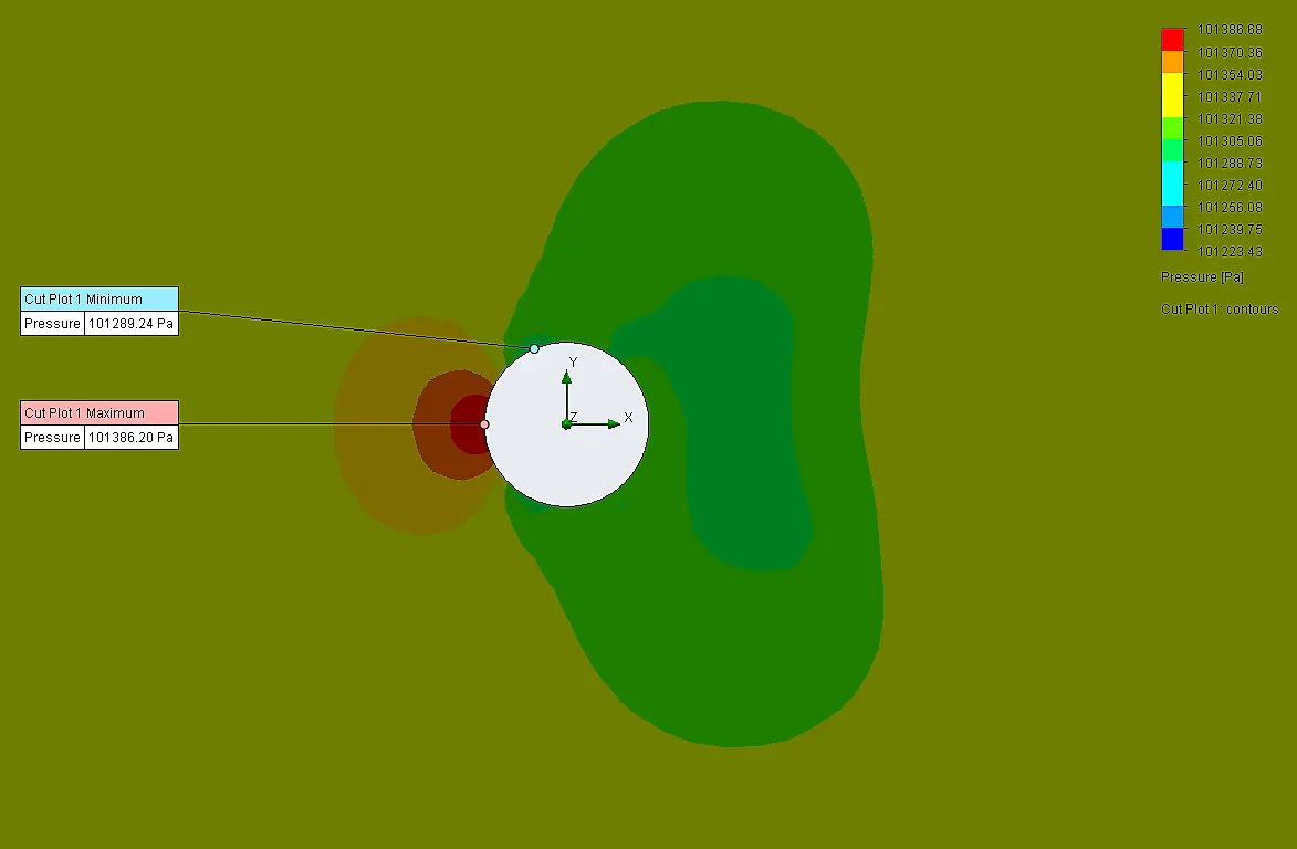
i. Due to this retardation of the flow at the front, the cylinder experiences a higher pressure on the surface facing the flow and lower pressure at the back. This difference of pressure exerts a force on the cylinder called as Pressure Force. The force experienced by the cylinder is a total drag force. this force has two components: Pressure Force and Viscous Force.
ii. In all the cases the surface exposed in the direction of the fluid flow experiences the large pressure force which is indicated as a red zone in the animation. the green zone shows the lower pressure on the cylindrical surface exposed in the flow direction of the fluid. the red zone is shown smaller because of the smaller area of impact while the green zone is larger due to the separation of the fluid from the surface of the cylinder.
iii. As Reynold's number increases the velocity increases and the flow-through time is decreased in all the cases. While in all the animation of the pressure, we can observe that the pressure changes are very small. Also, a flow changes from Laminar to Turbulent.
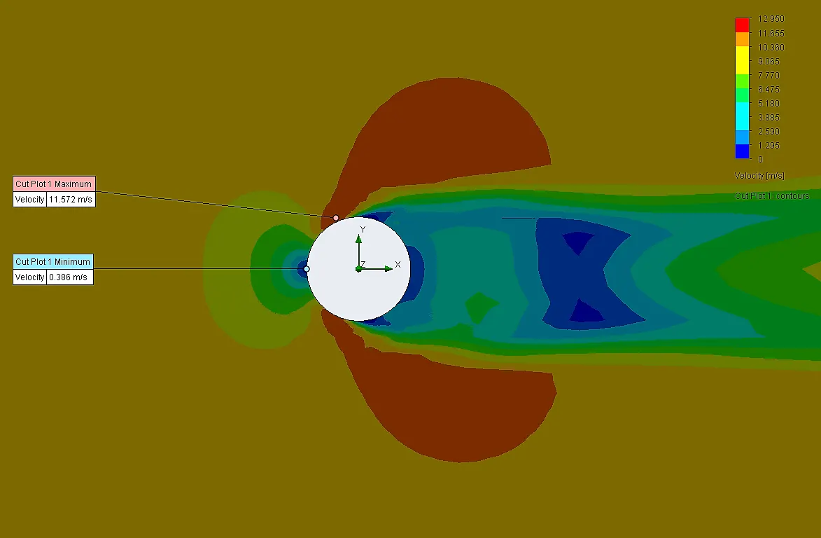
iv. Stagnation Point:- In the 'pressure view', we can see that the Red zone indicated as 'Cut plot 1 Maximum' and in the 'velocity view', we can see the blue region on the surface of the cylinder exposed to the fluid flow which is denoted as the 'cut plot 1 minimum'. These two regions indicate that the point where static pressure is maximum and velocity is minimum. Hence as we know that the point where velocity is minimum (near to zero) and static pressure is maximum is known as stagnation point.
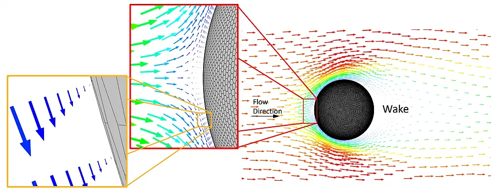
a stagnation point on the upstream surface where the flow comes to a
stop then turns and flows along the curvature of the sphere, accelerating in the process.
• Resolved boundary layer along the cylinder surface can be clearly seen.
• The Reynolds number is high enough for the flow to separate and form a wake downstream of the cylinder.
v. Separation Point and wake Region:- In the 'velocity view' we can see that the point is shown in red zone name as 'cut plot 1 maximum' is a point from where the separation of the fluid stream (or) boundary layer initiated. This is caused due to the boundary layer thickness affected by the pressure gradient also, separation takes place due to adverse (or) positive pressure gradient i.e when `(dp)/(dx)>0` and `(dv)/(dy)<= 0`
As we saw in the velocity view the flow separates from the surface and creating a highly turbulent region behind the cylinder called the wake.
Reference:
http://ecoursesonline.iasri.res.in/mod/page/view.php?id=1080