THE PIPE FLOW SIMULATION
1. Objective
1. Place line probes at 95%, 90%, and 85% of the pipe length.
2. Compare the normalized velocity profile at each of these locations.
3. Normalize the velocity profile by the inlet velocity.
2. Basic
The type of pipe flow can be determined with the help of the Reynold number. Also, the flow of fluid depends upon multiple parameters such as length of pipe, diameter of the pipe, nature of the fluid, share stress acting at the boundary and etc.
In the simulation, we will study the behavior of the fluid flowing inside a pipe. Here, our flowing fluid is water having a density of 1000 kg/m^3. Also, the type of flow (i.e Laminar or turbulent) is decided based on the Reynolds number. The formula for the Reynold number as follows.
`Re = (rho*V*D)/mu = (V*D)/nu` ....................................(i)
Where:-
ρ = Density of fluid
V = Velocity
μ = Viscosity
v = Kinematic Viscosity
D = Hydraulic Diameter (diameter of flowing fluid)
From the above formula, we can see that the Reynold number depends upon multiple parameters. based on those parameters the behavior of flowing fluid is can be determined. the fluid type based on the Reynolds number as follows.
Re < 2000 indicates Laminar Flow ;
Re = 2000 indicates Critical Flow ;
Re = 4000 indicates Transitional Flow ;
Re > 4000 indicates Turbulent Flow.
In our problem, we have three variable Reynolds numbers but we need to find out the velocities. So to do that we are going to use the above formula in the calculation section. Also to calculate the length we are going to take the help of Poisulle's Theorem-based formula as follows.
length from the entrance can be calculated based on the following formula.
`L=0.6⋅Re⋅D`...............................(ii)
Where:-
Re = Reynold number
D = Hydraulic diameter
3. Calculation
Before we are going to do a stepwise explanation we are going to calculate all the remaining parameters which are required in our analysis. We have three cases of Reynold number based on this we are going to find out the velocity and length of the pipe according to it. In all the cases we are going to take the external diameter of the pipe as 20mm and the thickness of the pipe as 1mm. Hence, the constant parameters taken are as follows.
D = 19mm (i.e 0.019 m)
ρ = 1000 kg/m^3 (for water)
μ = 0.001 (or) 8.90*10^-4 pa.sec
Note:- The unit system used in the simulation is MKS system.
3.1 Calculation of velocities:-
for all the Velocities below we are using equation (i).
a. For Case-1:
At Re = 100
`100=1000⋅V⋅0.0190.001`
`V= 0.005263`
b. For Case-2:
At Re = 1000
`1000 = 1000⋅V⋅0.0190.001`
`V = 0.005263`
c. For Case-3:
At Re = 10000
`10000=1000⋅V⋅0.0190.001`
`V= 0.5263`
3.2 Calculation of length:-
for all the length below we are using equation (ii).
a. For Case-1:
At Re = 100 ; L = 0.06*100*0.019 ; ;L = 114 mm
b. For Case-2:
At Re = 100 ; L = 0.06*1000*0.019 ; ;L = 1140 mm
c. For Case-3:
At Re = 100 ; L = 0.06*10000*0.019 ; ;L = 11400 mm
Final Calculation Table:-
| Reynold number | Velocity(m/s) | Length of pipe(mm) |
| 100 | 0.005263 | 114 |
| 1000 | 0.05263 | 1140 |
| 10000 | 0.5263 | 11400 |
4. Procedure & Explanation
Step-1:- Making pipe with a diameter of 20mm, Using Shell option for proving thickness to a pipe and making it hollow 1mm and a Varying length based on the calculation.
Step-2:- Making line probes at 95%, 90%, and 85% of the pipe length based on the following calculated table.
| Probe length at 95% | Probe length at 90% | Probe length at 85% | |
| Case-1 | 108.3 | 102.6 | 96.9 |
| Case-2 | 1083 | 1026 | 969 |
| Case-3 | 10830 | 10260 | 9690 |
Step-3:- Opening the flow simulation in the Solidworks. Before doing anything we need to seal the pipe from both sides to do that we used the Lid option.
Step-4:- Now after Sealing the pipe from both sides we are going to define the project in the flow simulation. To do that we are using the Wizard option and defined the basic parameters such as flow type, fluid type and etc which are the same for all three cases.
Step-5:- Defining the Boundary condition i.e Static pressure at the outlet, Inlet velocity at the inlet, and Real wall for the pipe body. the inlet velocities are different for different lengths which are shown in the table present in the calculation section.
Step-6:- Setting Mesh Manually X= 20 ; Y= 20 ; Z = 100 in all the cases for better result.
Note:- the mesh is differing according to the requirement, which is used in the parametric studies.
Step-7:- Setting Result. to do that we are going to plot XY-plots for velocities at each probe location. i.e probe present at 95%, 90%, and 85% of the pipe length. Also, we took common XY-plots for all the probe position. we defined the Result plots for the three cases and taken velocities according to the length of the pipe.
Step-8:- Creating Cut Plot near each probe location and making pipe transparent.
Step-9:- Doing parametric study to get the plot file and optimizing mesh and more. To do that we defined the X, Y, and Z mesh as an input parameter. similarly, the output parameter is All the plots and in the scenario, we increase the mesh size. We did this study in all three cases.
Note:- In the scenario, we did multiple studies at increased mesh size but not showing the increase in the size of the mesh here. We only Display the plot which is more clear to understand and enough for comparison between the three cases.
5. Simulation and Analysis
In this, we are going to plot the different results and compare them. the comparison as shown below for each probe for different cases.
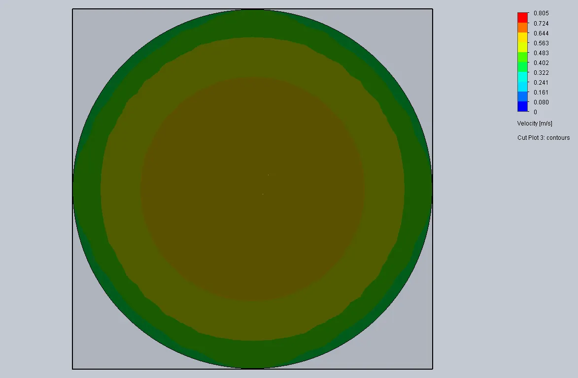
5.1. Cut plot at Different probe location in three Cases:-
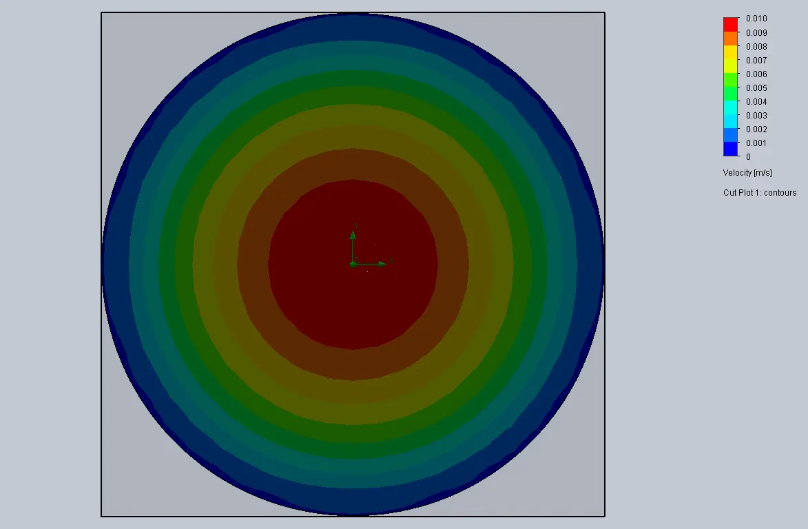
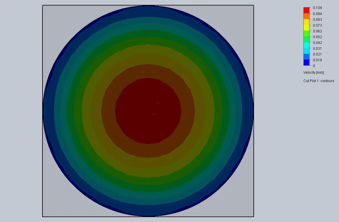
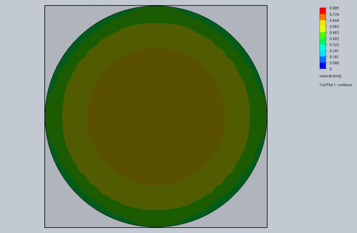
5.1.1 At probe 1:- Cut plots at 95% of the length in the three cases.
Case-1
Case-2
Case-3
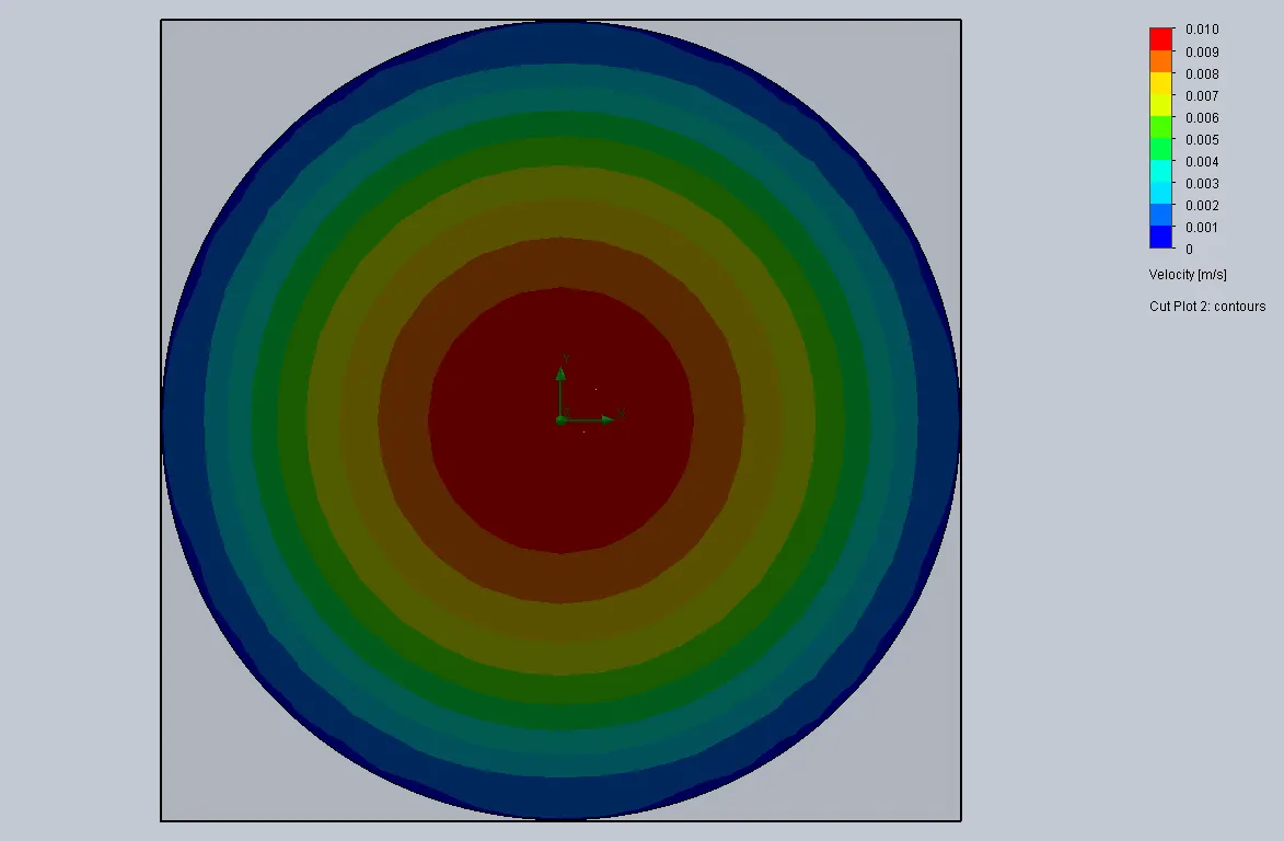
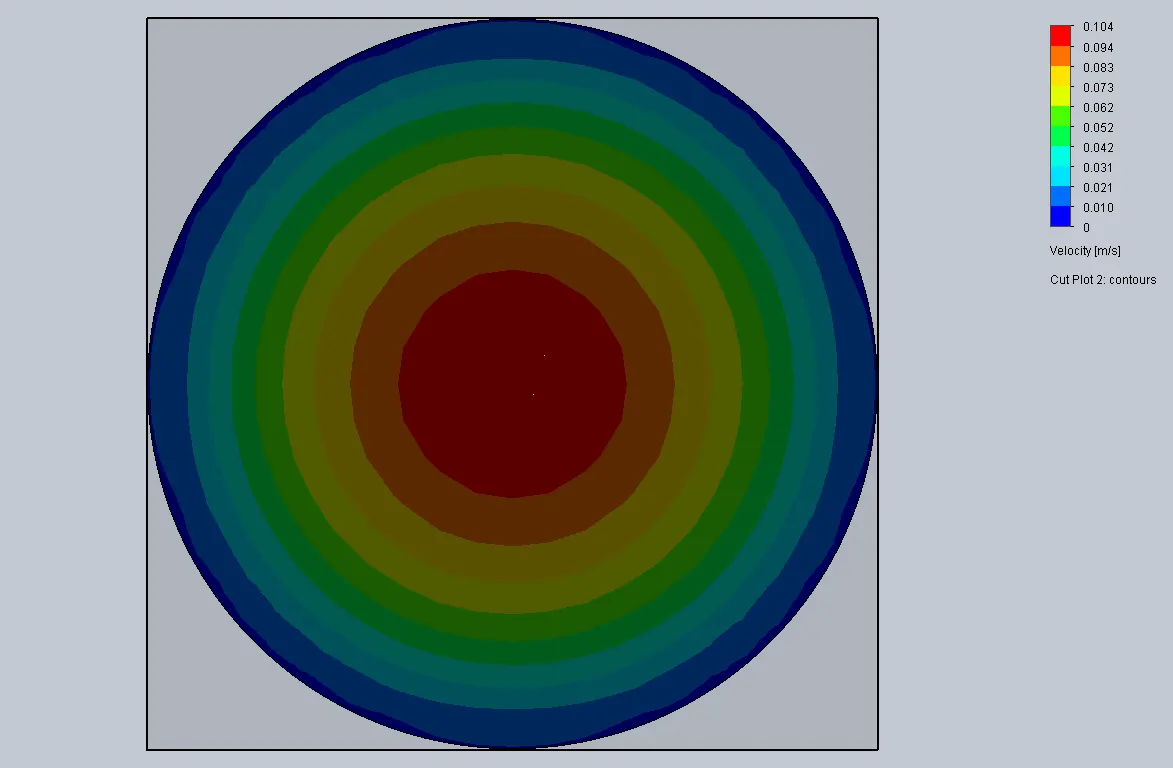
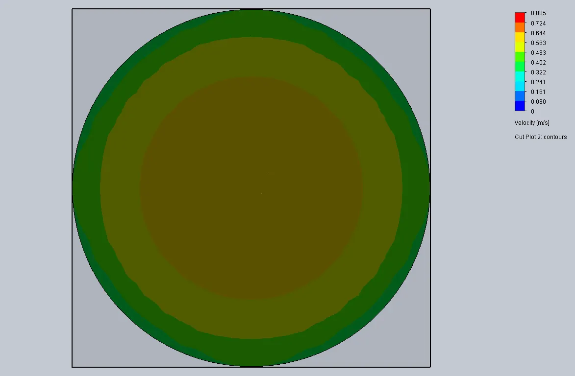
5.1.2 At probe 2:- Cut plots at 90% of the length in the three cases.
Case-1
Case-2
Case-3
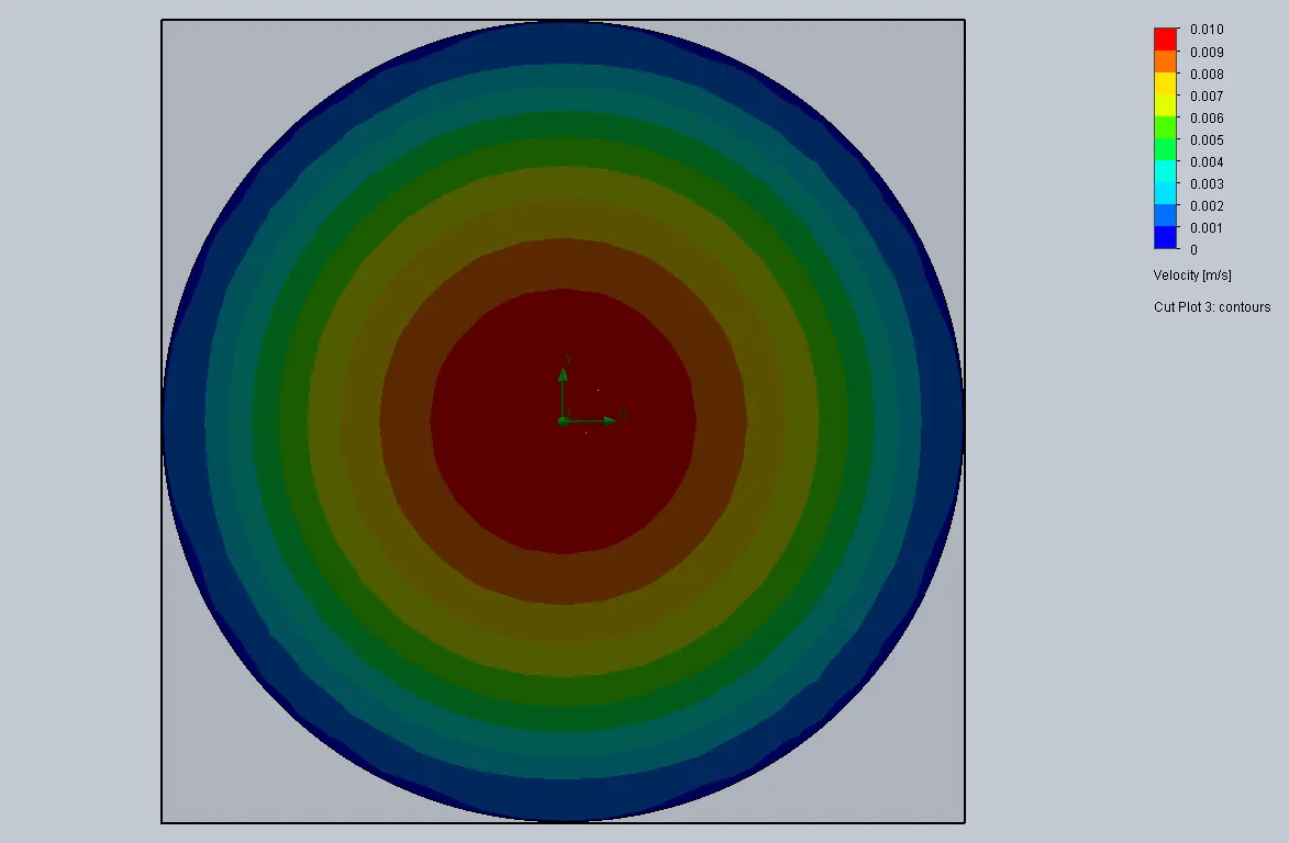
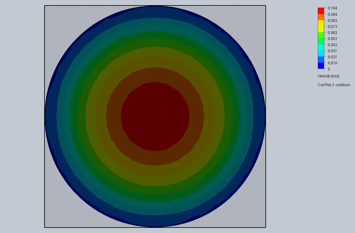
5.1.3 At probe 3:- Cut plots at 85% of the length in the three cases.
Case-1
Case-2
Case-3
5.2 Velocity Plot at Different probe location in three Cases:-
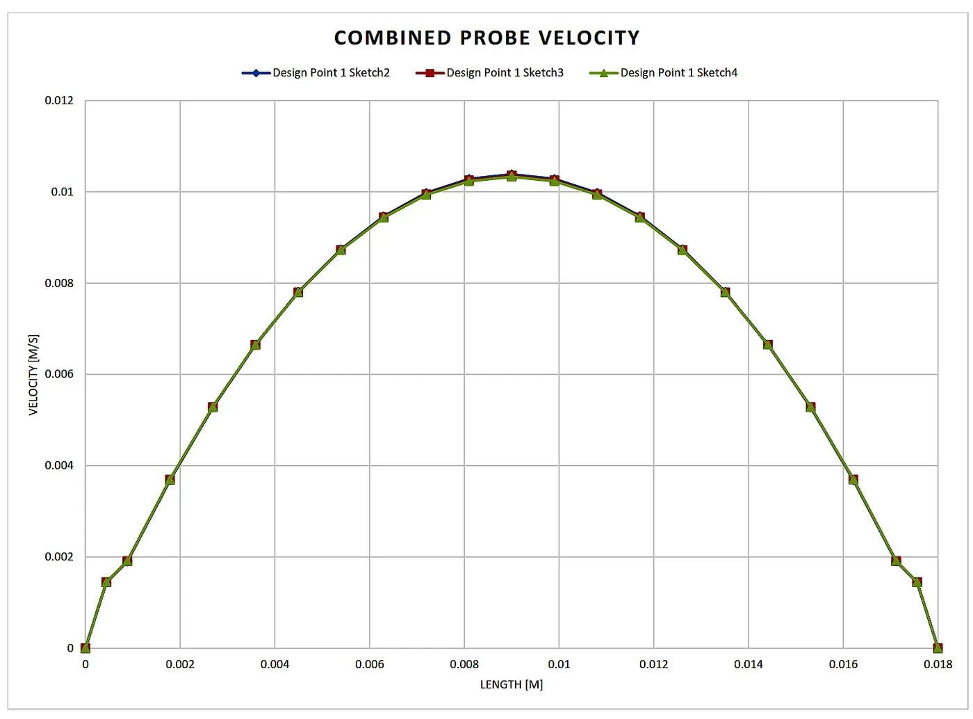
5.2.1 Velocity at 95%, 90%, and 85% of the Pipe length for the first case:-
Parabolic Profile Due to Laminar flow.
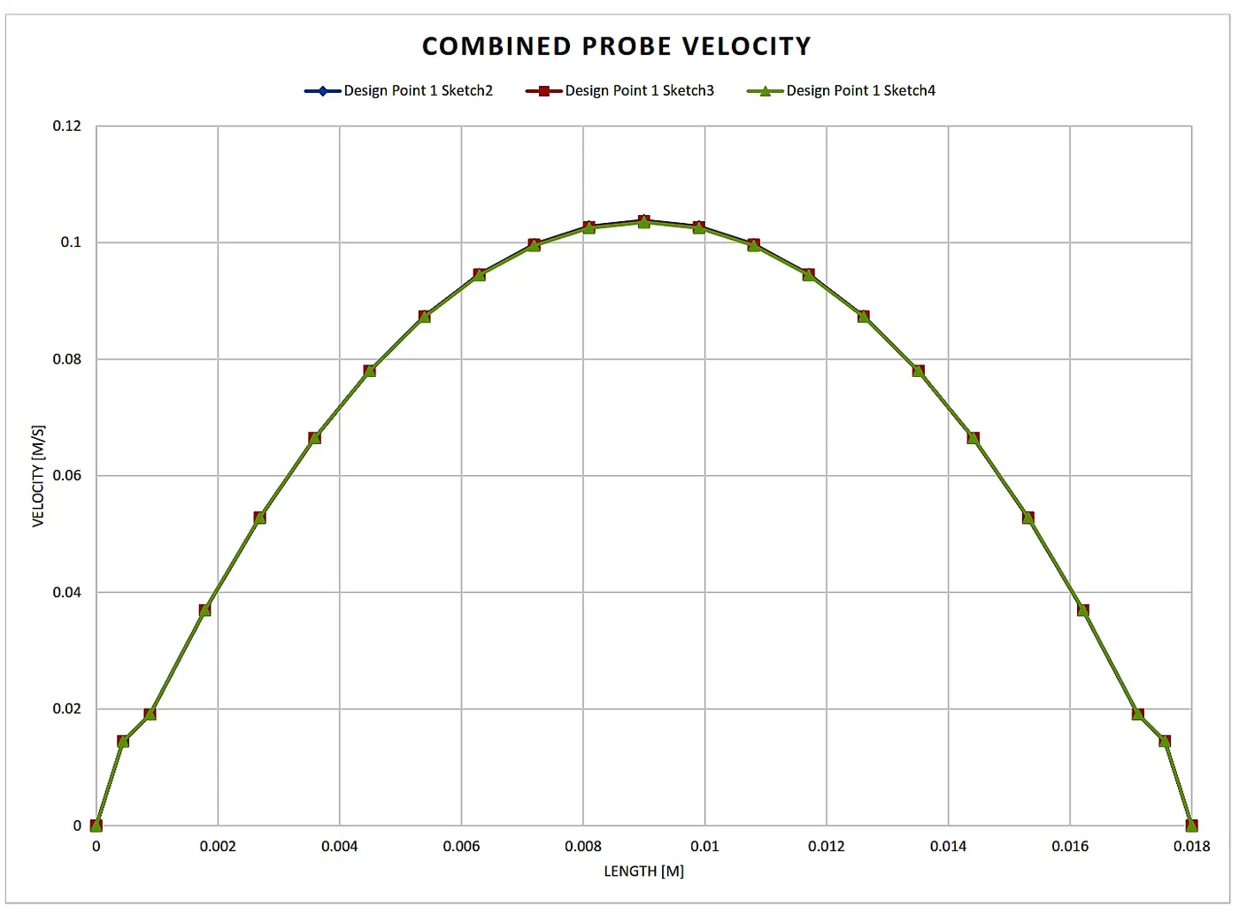
5.2.2 Velocity at 95%, 90%, and 85% of the Pipe length for the Second case:-
Parabolic Profile Due to Laminar flow.
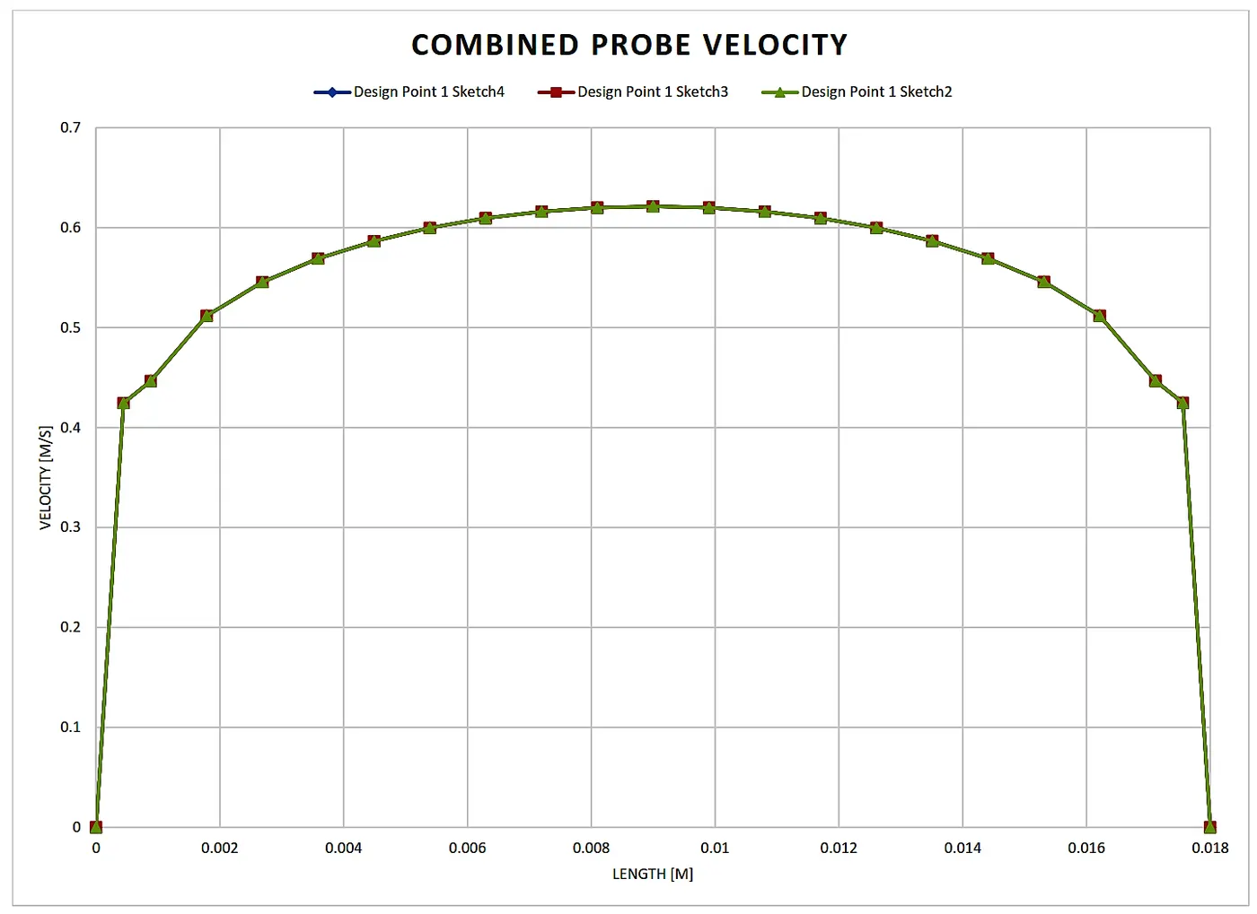
5.2.3 Velocity at 95%, 90%, and 85% of the Pipe length for the third case:-
Logarithmic Profile due to Turbulent Flow.
5.3 Comparing all the three Cases Plot:-
To compare all the results of the three cases, we are Superimposing the graph as follows which indicates that the change of flow type from Laminar to Turbulent based on the velocity profile.
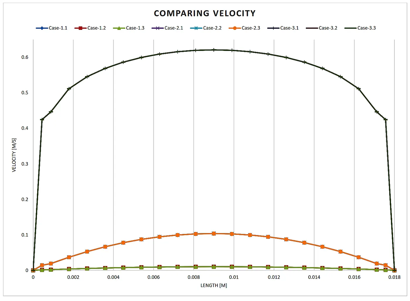
(the comparison is discussed in the conclusion section.)
6. Conclusion
1. The Plot of Case-1 and Case-2 indicates the velocity profile is parabolic in nature in which the initial and final velocities are minimum at the pipe boundary and maximum at the Middle. This is caused due to the Share stress acting at the wall is maximum and at the middle share, stress is minimum.
2. Also in case-1 and case-2, the Reynolds number is lower i.e 100 and 1000 respectively. the flow in the pipe is Laminar.
3. The plot of case-3 of the velocity profile is not parabolic i.e it is a Logrithemic. as the Reynolds number is Higher i.e 10000 the flow is Turbulent.
4. The probe used in our study indicates that the small velocity variation before the length of fully developed flow. i.e as the fluid is flowing in the pipe the velocity changes unlit the flow is fully developed after that the velocity in the pipe is constant. The length about which the flow is getting fully developed is based on Poisulle's Theorem.
5. As the Reynolds number increases the velocity in the pipe and length of pipe to fully developed flow is increases. also, the velocity profile changes indicate that the change in flow from Laminar to turbulent as shown in the last combined velocity plot of all the three cases. Hence, we can conclude that the type of flow depends upon the Reynolds number.