FORWARD KINEMATICS OF A 2R ROBOTIC ARM.
1. Objective:-
i. To write a program in Matlab and python to simulate the forward kinematics of a 2R Robotic Arm.
ii. Create an animation file of the plot.
2. Basic:-
2.1 Concept of kinematics:
In Kinematics only Velocity and Acceleration Analysis of various parts it to be done. Forces are neglected.
2.2 The origin of Robotics and linking with Human:
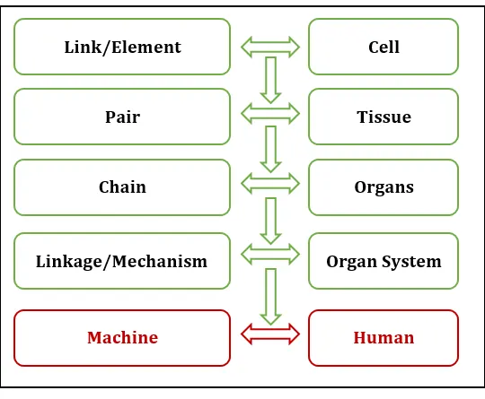
The links are the smallest unit of the Machine, similar to the cell in the Human Body. By a combination of the link, pair is formed and pair together forms a chain and which further causes linkage formation, and at last, the combination of Linkage (also known as Mechanism) forms Machine. The Machine is the basis of the Robotics. The simplest explanation for the origin of Robotics/Machine and linking with Humans is as follows.
2.3 Mechanical linkage:-
A mechanical linkage is an assembly of bodies connected to manage forces and movement. The movement of a body, or link, is studied using geometry so the link is considered to be rigid. The connections between links are modelled as providing ideal movement, pure rotation, or sliding for example, and are called joints. A linkage modelled as a network of rigid links and ideal joints is called a Kinematic chain. For example, The basic linkage mechanism in practice is a deployable mirror linkage constructed is shown below.
2.4 Approach:-
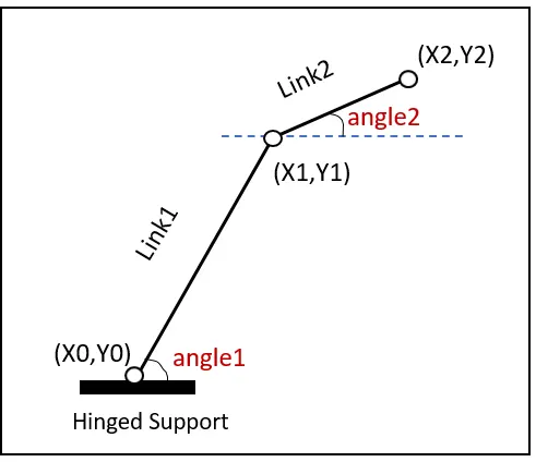
In our Project, we are going to use the basic arms of the robot to do that we are dealing with the linkage known as Forward kinematics of a 2R Robotic arm (where 2R means 2-rotating Link i.e 2 is a number of link and R is rotation). we are taking two links as a representative of the Robotic arm in which Link-1 is Hinged at (X0, Y0) and making an angle1, while Link-2 is hinged at the end of the Link-1 and making angle2 with respect to Datum.
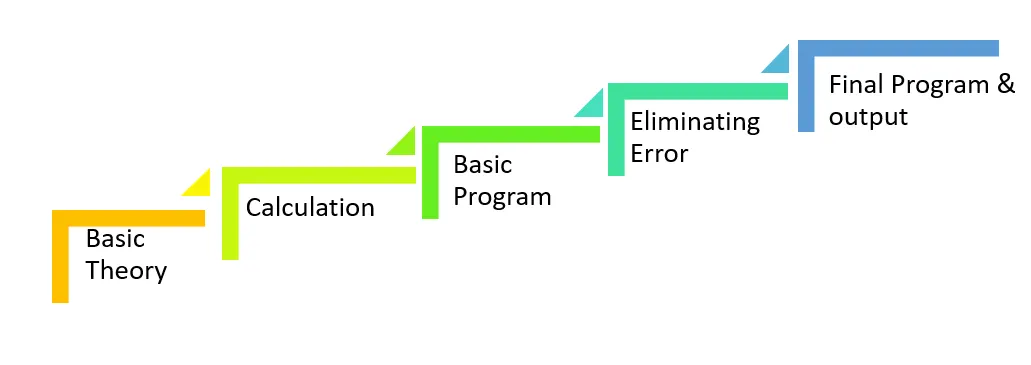
We need to Animate the Arm and find out its behavior in Different conditions. Our Approach to Get the final Program and a series of steps that we will perform during the entire Problem is shown below in the Step chart.
3. Detailed Procedure and Explanation:-
3.1 Procedure and Explanation for Matlab:
Step-1: Calculating the position of Link-1.
From the fixed Support, the initial value of X and Y for the Link-1 (X0, Y0) and the final value is (X1, Y1)
X0=0
Y0=0
X1= L1* cosd(A1)
Y1 =L1* sind(A1)
Step-2: Calculating the position of the Link-2.
For the Link-2 starting point is the Ending point if the Link-1 ie (X1, Y1) and Ending point is (X2, Y2)
X2 = X1+l2* cosd(A2)
Y2 = Y1+l2* sind(A2)
Step-3: Writing Basic Program.
Basic Program represents the basic idea about the plot where we get only 2D plot but no animation.
To get the basic plot first We are Providing the basic input as L1= 2 and L2=1
In meters also angle1 = 45 and angle2 = 30 in degree
a1=angle1; a2=angle2;
And providing basic condition as above in step-1 and step-2, and for plotting we are using the command Line not plot because plot command gives us an error
Line ( [ X0 X1 ], [ Y0 Y1 ] )
Similarly,
Line ( [ X1 X2], [Y1 Y2] )
close all
clear all
clc
%  Program for the kinematices of robotices arm
%inputs
l1 = 1
l2 = 0.5

angle1=45
angle2=30

A1 = angle1
A2= angle2

%coordinates
x0=0
y0=0

x1 = l1* cosd(A1)
y1 = l1* sind(A1)

x2 = x1+l2* cosd(A2)
y2 = y1+l2* sind(A2)

line([x0 x1], [y0 y1],'linewidth', 3, 'color' ,'r')
line([x1 x2], [y1 y2],'linewidth', 3, 'color' ,'b')
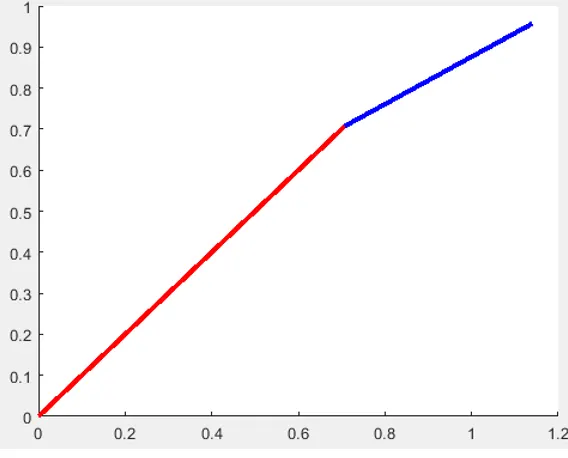
The output of the Programm is a simple plot as shown below.
But in this, we are not getting the animated plot to do that we are using a separate program in the next step.
Step-4: Program for Arm Animation and Error Elimination.
Here we are taking multiple angles and multiple values of (X, Y).
Initially, we are providing the inputs for the angle with the help of linspace command as follows
Angle1 = linspace (0 , 90, 10)

Angle2 = linspace (0, 90, 10)
Where:-
In linsapce command the first value represents the starting point of angle, similarly, the second point represents the ending point of the angle and at last, the third point represents the number of values between them
To change the angle we are using For-loop command as shown below.
for i = 1: length(angle2)

ANGLE1 = angle1(i)
ANGLE2 = angle2(i)

a1=angle1;
a2=angle2;
Now, here is the value of (i) changes we are taking the values of angle1, angle2 from the original arrays, and assigning to the variable called ANGLE1, ANGLE2.
We use the value of (i) to take particular value for angle1 and angle2 and then we are going to perform forward kinematics calculation hence, rearrange Program in the following manners. for each value of angle1, each position of the link1, link2 can take multiple positions and which is depend's on angle2.
Further, if it is ANGLE1 then ANGLE2 required another for-loop. for each value of angle1, we are looping the value of angle2, which is as follows.
for i = 1: length(angle1)
A1=a1(i)                      % i.e ANGLE1 = angle1(i)

for j = 1: length(angle2)
A2=a2(j);                    % i.e ANGLE2 = angle2(j)
End
for kinematic calculation, we are copying our first program below the line ANGLE2 = angle2(j) and change the angle to ANGLE accordingly as follows.
x0=0;
y0=0;

x1 = l1* cosd(A1);
y1 = l1* sind(A1);
x2 = x1+l2* cosd(A2);
y2 = y1+l2* sind(A2);

%plotting
line([x0 x1],[y0 y1])
line([x1 x2],[y1 y2])
we got our first plot but not animation as follows.
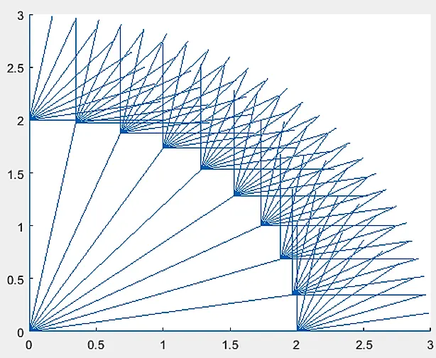
To eliminate this we are typing figure(ct) before plotting and outside for-loop ct=1
And after the plot command type ct=ct+1 (i.e we incrementing the value each time program gets executed in the for-loop) and executing the command we get 100 independent plots (because our angle1 value is 10 and angle2 value is also 10).
Therefore to get rid of this we are using plot command instead of line command.
line([x0 x1],[y0 y1])
line([x1 x2],[y1 y2])
Again we get the same result but most recent link as a plot result. To prevent this we are using hold on and pause command. Here we get the result as a 1st result (error) but animated.
Now we are going to remove the 2nd plot command and make the first plot as below
plot([x0 x1],[y0 y1],[x1 x2],[y1 y2])
we get an animated plot with random color changes as shown below.
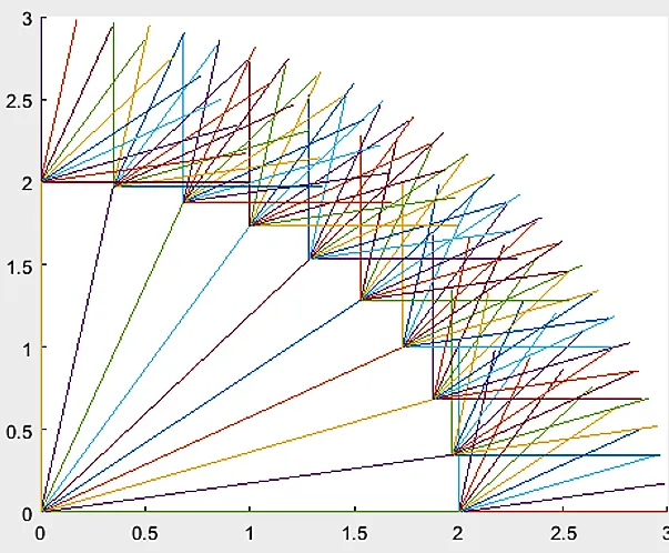
Now removing hold on command and including the axis command, adjusting the pause interval is gives us the better result.
for axis([-0.3 3.6 -0.3 3.6]) and for pause interval as pause (0.1). we get our Required Result but further, we need to make a movie of it, which is in next step.
Step-5: Creating a movie.
To create movie type M(ct)=getframe(gcf) just below the pause(0.01) and at extreme end command type Movie(M)
Where:- ct represents every frame and getfram command represents to getting the current figure in the gcf window. Further, we are going to save all the figures in the array called (M).
Further, we are creating avi file to get this we are using following commands.
videofile = VideoWriter('forward_kinematics.avi');
open(videofile)
writeVideo(videofile, M)
close(videofile)
Note:- while using the writeVideo command use it as it is because it is case sensitive hence any mistake can give an error in the program execution. Also, we can use uncompress command but it gives us the large avi file. Hence in this program, we are not using it.
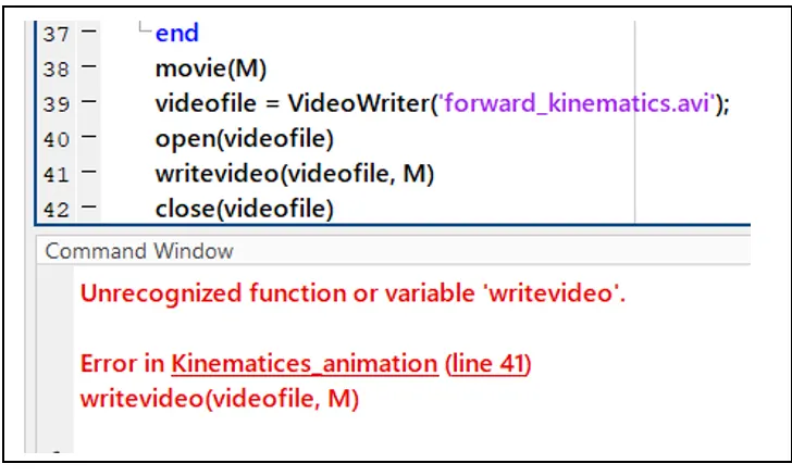
The final program is as shown below:
clear all
close all
clc

% Inputs
l1=2;
l2=1;
angle1 = linspace(90,0,10);
angle2 = linspace(90,0,60);
a1=angle1;
a2=angle2;

ct=1;
for i= 1:length(a1) %represents the no of value in angle1
    A1=a1(i);
    for j= 1 : length(a2)
        A2=a2(j);
x0=0;
y0=0;

x1 = l1* cosd(A1);
y1 = l1* sind(A1);

x2 = x1+l2* cosd(A2);
y2 = y1+l2* sind(A2);

%plotting

plot([x0 x1],[y0 y1],[x1 x2],[y1 y2],'linewidth', 3);

axis([-0.3 3.6 -0.3 3.6])
pause(0.01);
M(ct)=getframe(gcf);
ct=ct+1;

    end
end
movie(M)
videofile = VideoWriter('forward_kinematics.avi');
open(videofile)
writeVideo(videofile, M)
close(videofile)
3.2 Procedure and Explanation for Python:
Step-1: Before doing the program we are using the import command to import the libraries which will use for mathematical operation and plotting.
import math
import matplotlib.pyplot as plt
The "import math" and "import matplotlib.pyplot as plt" are used to use the mathematical constants and plotting the graph respectively.
Step-2: Defining input parameters such as length of the first and second link, number of values of theta, starting angle, and ending angle. Here we need to start the link from zero degrees angle and end with the 90 degrees.
# Inputs
l1 = 1
l2 = 0.5
n_theta = 10
theta_start = 0
theta_end = (math.pi)/2
Assigning the individual values for theta is not convenient and time-consuming hence we defined the n_theta = 10 for getting the 10 values of theta.
Step-3: We defined the theta1 and theta2 as an empty array. Because for Animating the plot we need to get the range of values for theta1 and theta2. Hence to get multiple values of theta1 and theta2 we need to use for-loop. the multiple values will generate and get store in the empty array. the for-loop is as shown below.
for i in range (0,n_theta):
	tmp = theta_start + i*(theta_end- theta_start)/(n_theta-1)
	theta1.append(tmp)
	theta2.append(tmp)
Where:-
i. For loop use to repeat the set of actions multiple times.
ii. we are taken arbitrary alphabet (i) which is acts as a loop counter. defining its range from zero to n_theta.
iii. The " theta_start + i*(theta_end- theta_start)/(n_theta-1) " used because when each time loop let executed the value of theta get updated to new value.
iv. ".append" is used to continuously append (increase) the value of the tmp and store it in the empty array.
Step-4: Defining the position of the links and using it in the new for-loop.
position of Link-1:
From the fixed Support, the initial value of X and Y for the Link-1 (X0, Y0) and the final value is (X1, Y1)
x0 = 0
y0 = 0
x1 = x0 + l1*math.cos(t1)
y1 = y0 + l1*math.sin(t1)
position of the Link-2:
For the Link-2 starting point is the Ending point if the Link-1 ie (X1, Y1) and Ending point is (X2, Y2)
x2 = x1 + l2*math.cos(t2)
y2 = y1 + l2*math.sin(t2)
For each value of the theta1 and theta2, we are going to plot. so to do that we need another for-loop. In the for-loop, we are going to use the position of link-1 and link-2 to get multiple combinations of value.
for t1 in theta1:
	for t2 in theta2:

		#link 1 and link 2 connetor
		x1 = x0 + l1*math.cos(t1)
		y1 = y0 + l1*math.sin(t1)

		# Manipulator coordinate
		x2 = x1 + l2*math.cos(t2)
		y2 = y1 + l2*math.sin(t2)
Step-5: Finalizing program.
filename  = str(ct) + '.png'
ct =ct+1

plt.figure()
plt.plot([x0,x1],[y0,y1])
plt.plot([x1,x2],[y1,y2])
plt.xlim([0,2])
plt.ylim([0,2])
plt.savefig(filename)
To generate the file name and we defined the (ct) as a loop counter out of the for loop and ct+1 inside for-loop to update the name of the file each time for-loop get executed. converting the integer to string.
using plot command to define the axis limit, plot the figure, and save it on the computer.
The final program is as shown below:
import math
import matplotlib.pyplot as plt

# Inputs
l1 = 1
l2 = 0.5
n_theta = 10
theta_start = 0
theta_end = (math.pi)/2
theta1 = []
theta2 = []

for i in range (0,n_theta):
	tmp = theta_start + i*(theta_end- theta_start)/(n_theta-1)
	theta1.append(tmp)
	theta2.append(tmp)

x0 = 0
y0 = 0

ct = 1
for t1 in theta1:
	for t2 in theta2:

		#link 1 and link 2 connetor
		x1 = x0 + l1*math.cos(t1)
		y1 = y0 + l1*math.sin(t1)

		# Manipulator coordinate
		x2 = x1 + l2*math.cos(t2)
		y2 = y1 + l2*math.sin(t2)

		filename  = str(ct) + '.png'
		ct =ct+1

		plt.figure()
		plt.plot([x0,x1],[y0,y1])
		plt.plot([x1,x2],[y1,y2])
		plt.xlim([0,2])
		plt.ylim([0,2])
		plt.savefig(filename)
4. Result and Conclusion:-
i. Output in Matlab:
ii. Output in Python: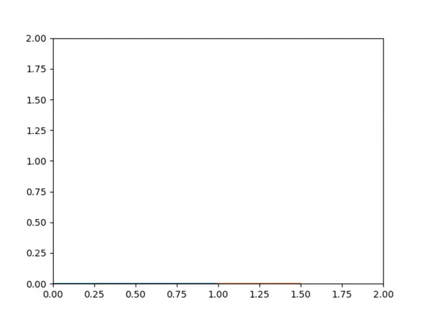
Note:- In the case of Python we created the animation by combining the png file of different Movement of the arm at different locations.
4.1 Conclusion:
Hence, We are able to Program the 2R robotic Arm, with the help of this program. By small adjustments in the program, we can use it in multiple applications. such as in case of Matlab, By changing the Data in the above lines and small adjustments in the program we can get multiple outputs such as we can move the arm in multiple directions and multiple speeds
angle1 = linspace(90,0,10);
angle2 = linspace(90,0,60);
Also, we can get multiple outputs such as we can move the arm in multiple directions and multiple speeds, also we can able to make the new program such as 3R robotic arm Simulation.
Reference:-
The flow of Report:-
1. Objective.
2. Basic.
3. Detailed Procedure and Explanation.
4. Result & Conclusion.