Analysis On A Plate With A Hole
1. Objective:-
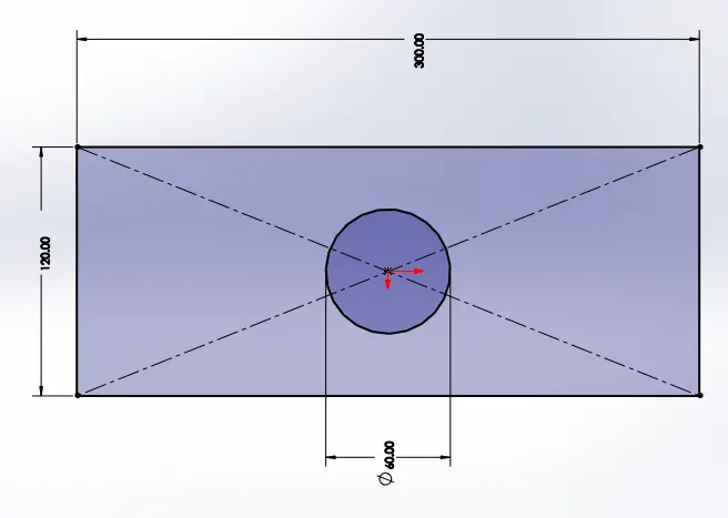
To Perform a static analysis on two models of a plate with holes. (Axial Loading).
create the model in Solidworks and perform the analysis using the following parameters table.
| CASE-1 | CASE-2 |
| Length=300mm | Length=300mm |
| Height=120mm | Height=120mm |
| Thickness=30mm | Thickness=30mm |
| Circular Hole at the center Diameter=60mm |
Circular Hole at the center Diameter=60mm |
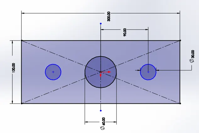
| -----------------NA------------------- | Two holes of 30 mm diameter which are placed 90mm away from the central hole on both sides. |
Apply a fixed relation to one of the short sides of the plate and apply a force of 1000N on the other such that the plate is stretched.
Run the analysis and compare the results for stress, strain, and displacement.
Describe the findings in a detailed report.
2. Basics:-
Various methodologies are developed to get the best advantages from the material to produce an optimized product. Stress calculation becomes a vital part of this process to design a product that won't break or deform. Geometrical discontinuities such as notches, holes should be considered as they make the component weaker. These geometrical discontinuities in the component lead to stress concentration in the localized area.
2.1 Geometric Irregularities:
- A sudden change in the cross-sectional area of a component is called a geometric discontinuity. such as hole, keyways, Notch, slot, groove, sharp etc.
- Cracks created during the manufacturing process are called surface non-homogeneity.

2.2 Concept of Stress Concentration:
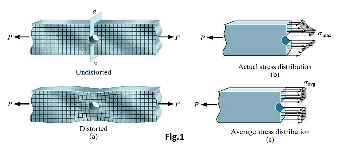
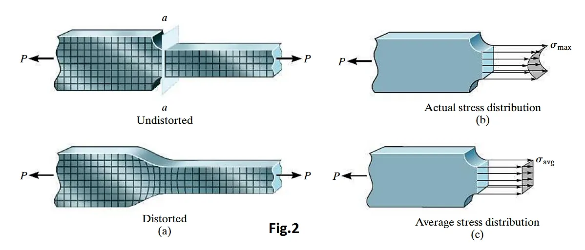
When an axial force is applied to a member, it creates a complex stress distribution within the localized region of the point of load application. Not only do complex stress distributions arise just under a concentrated loading, but they can also arise at sections where the member’s cross-sectional area changes. For example, consider the bar in Fig.1 a, which is subjected to an axial force P. Here the once horizontal and vertical grid lines deflect into an irregular pattern around the hole centered in the bar. The maximum normal stress in the bar occurs in section a – a, which is taken through the bar’s smallest cross-sectional area. Provided the material behaves in a linear-elastic manner, the stress distribution acting on this section can be determined either from mathematical analysis, using the theory of elasticity, or experimentally by measuring the strain normal to section a – a and then calculating the stress using Hooke’s law, `[sigma= E*epsilon]`. Regardless of the method used, the general shape of the stress distribution will be as that shown in Fig.1 b. Similarly, if the bar has a reduction in its cross-section, achieved using shoulder fillets as in Fig.2 a, then again the maximum normal stress in the bar will occur at the smallest cross-sectional area, section a – a, and the stress distribution will look like that shown in Fig.2 b. In engineering practice, the actual stress distributions in Fig.1 b and Fig.2 b do not have to be determined. Instead, only the maximum stress at these sections must be known, and the member is then designed to resist this stress when the axial load P is applied.
Specific values of this maximum normal stress can be determined by experimental methods or by advanced mathematical techniques using the theory of elasticity. The results of these investigations are usually reported in graphical form using a stress-concentration factor K. We define K as a ratio of the maximum stress to the average normal stress acting at the cross-section; i.e.,
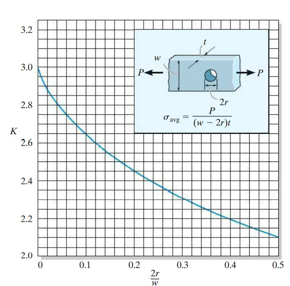
Specific values of K are generally reported in handbooks related to stress analysis. Note that K is independent of the bar’s material properties; rather, it depends only on the bar’s geometry and the type of discontinuity. As the size r of the discontinuity is decreased, the stress concentration is increased. the maximum normal stress will be three times greater than the average normal stress on the smallest cross-section.
2.3 The theoretical stress concentration factor:
The theoretical stress concentration factor can be calculated with the handbook data.
the data is based on the diameter of the hole and width of the plate.
this data can be used for a plate with a hole subjected to uniaxial loading.
The stress-concentration factors given in were determined on the basis of static loading, with the assumption that the stress in the material does not exceed the proportional limit. If the material is very brittle, the proportional limit may be at the fracture stress, and so for this material, failure will begin at the point of stress concentration. Essentially a crack begins to form at this point, and a higher stress concentration will develop at the tip of this crack. This, in turn, causes the crack to propagate over the cross-section, resulting in a sudden fracture. For this reason, it is very important to use stress concentration factors in design when using brittle materials. On the other hand, if the material is ductile and subjected to a static load, it is often not necessary to use stress-concentration factors since any stress that exceeds the proportional limit will not result in a crack. Instead, the material will have reserve strength due to yielding and strain hardening. In the next section, we will discuss the effects caused by this phenomenon.
Stress concentrations are also responsible for many failures of structural members or mechanical elements subjected to fatigue loadings. For these cases, a stress concentration will cause the material to crack if the stress exceeds the material’s endurance limit, whether or not the material is ductile or brittle. Here, the material localized at the tip of the crack remains in a brittle state, and so the crack continues to grow, leading to a progressive fracture. As a result, one must seek ways to limit the amount of damage that can be caused by fatigue.
2.4 Methods to reduce stress concentration:
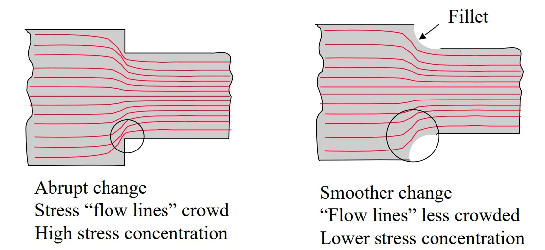
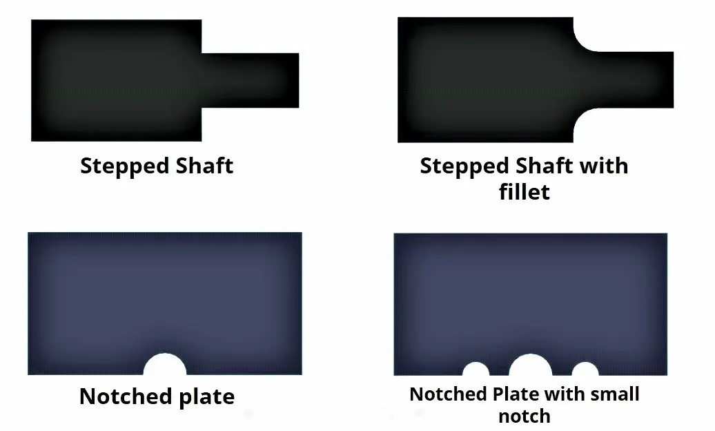
- Adding Fillets - cross-sectional may vary gradually
- Adding grooves and small notches will reduce stress concentration.
2.5 Examples:
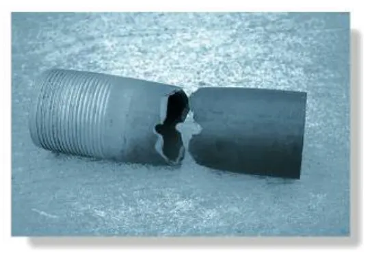
1. Failure of this steel pipe in tension occurred at its smallest cross-sectional area, which is through the hole. Notice how the material yielded around the fractured surface.
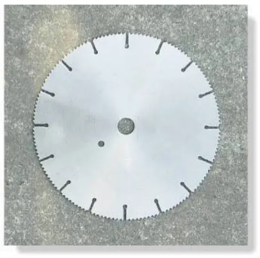
2. This saw blade has grooves cut into it in order to relieve both the dynamic stress that develops within it as it rotates and the thermal stress that develops as it heats up. Note the small circles at the end of each groove. These serve to reduce the stress concentrations that develop at the end of each groove.
3. Calculation:-
3.1 Formula:
Stress concentration factor can be calculated based on the following formula.
`[K_t= sigma_max/sigma_(nom)]`
Where:-
`K_t` = Theoretical Stress concentration factor
`sigma_max` = Maximum stress
`sigma_(nom)` = Nominal stress is Average stress in a component having uniform cross-sectional maximum stress- stress occurred due to discontinuity.
The stress is calculated based on the elastic theory is called nominal stress. where in the elastic theory we assume that the material obeys the hooks law.
3.2 Calculating the maximum stress through the theoretical stress concentration factor:
we know that `[K_t= sigma_max/sigma_(nom)]`
hence, `sigma_max= K_t*sigma_(nom)`
To calculate the max stress we need to calculate first the nominal stress based on the following formula.
`sigma_(nom)=F/A`
Where:-
`A=(w-d)⋅t)`
`F` = load
`W` = width
`d`=dia for a hole
`t` = thickness of the plate
3.2.1 The calculation for Case-1:
a. Calculating Nominal Stress:
Because `sigma_(nom)=F/((w-d)⋅t)`
`sigma_(nom)=1000/((120-60)*30)`
`sigma_(nom)=0.56` Mpa
b. Calculating D/W ratio:
we need to find out Value to stress concentration factor from Graph.
Therefore, we need a D/W ratio.
Hence,
So, from the graph, the value of stress concentration factor for 0.5 D/W ratio is 2.1.
Hence `K_t= 2.1`
c. Calculating Theoretical Maximum Stress:
because `sigma_max= K_t*sigma_(nom)` becomes
hence, `sigma_max= (2.1)*(0.56) = 1.176`
3.2.2 The calculation for Case-2:
a. Calculating Nominal Stress:
Because `sigma_(nom)=F/((w-d)⋅t)`
therefore for three holes,
`sigma_(nom)=1000/[((120-60)+(120-30)+(120-30))*30]`
`sigma_max=0.1389` Mpa
b. Calculating D/W ratio:
we need to find out Value to stress concentration factor from Graph as we discussed in case-1.
Therefore, we need a D/W ratio.
Hence, `D/W = 30/120 = 1/4=0.25`
So, from the graph, the value of stress concentration factor for 0.25 D/W ratio is 2.4.
Hence `K_t= 2.4`
But in this case, we have three holes in the plate out of which the dimension of a larger hole is the same as the case-1 so the theoretical stress concentration factor for this hole is the same as before. i.e `K_t = 2.1` . and for remaining, 2 holes have `K_t=2.4`
Hence overall theoretical stress concentration factor is as follows.
`K_t = 2.1+2.4+2.4 = 6.9`
c. Calculating Theoretical Maximum Stress:
because `sigma_max= K_t*sigma_(nom)` becomes
hence, `sigma_max= (6.9)*(0.1389) = 0.95841` Mpa
3.3 Analytical Method:
Other than the graphical method we can calculate the theoretical stress concentration value using the Analytical Method as discussed below.
`K_t= 3- 3.14*(D/W)+3.667*(D/W)^2-1.527*(D/W)^3`
1. for case -1:
`K_t = 3-3.14(0.5)+ 3.667(0.5)^2- 1.527(0.5)^3`
`K_t= 2.115`
hence,
`sigma_max = (2.115)*(0.56) = 1.1844` Mpa
1. for case -2:
As we know we have three holes in the plate out of which the major hole has the same diameter as case-1. so that stress concentration value for this hole is `K_t= 2.115`.
we need to calculate the stress concentration value for the other two holes.
hence, stress concentration value for the 30mm diameter holes having D/W ratio is 0.25.
`K_t = 3-3.14*(0.25)+3.667*(0.25)^2-1.527(0.25)^3`
`K_t = 2.419890`
therefor, Overall value is `K_t = 2.155+2.419890+2.419890 = 6.9947`
Hence, `sigma_max = (6.9947)*(0.1389) = 0.97156383` Mpa
4. Simulation and Analysis:-
Now we are going to find out the maximum stress using the SolidWorks simulation, Validating it with our theoretically calculated value and finding error in between the results.
The material properties are the same for all the cases which are as follows.
Material Properties:
| Property | Value | Units |
| Elastic Modulus | 210000 | N/mm^2 |
| Poisson's Ratio | 0.28 | N/A |
| Shear Modulus | 790000 | N/mm^2 |
| Mass Density | 7700 | kg/m^3 |
| Tensile Strength | 723.8256 | |
| Compressive Strength | N/mm^2 | |
| Yield Strength | 620.422 | N/mm^2 |
| Thermal Expansion Coefficient | 1.3e-05 | /K |
| Thermal Conductivity | 50 | W/(m/k) |
| Specific Heat | 460 | j/(kg.k) |
| Material Damping Ratio | - | - |
Other parameters:
| Model Type | : Linear Elastic Isotropic |
| Units | : SI-N/mm^2 (Mpa) |
| Category | : Steel |
| Name | : Alloy Steel |
| Default Failure Criterion | : Max von Mises Stress |
| Sustainability | : Defined |
4.1 Case-1:
Step-1: Designing the plate with hole based on the dimension provided as shown below.
Step-2: Defining a new study as a static analysis
Step-3: Apply a fixed relation to one of the short side of the plate and apply a force of 1000N on the other such that the plate is stretched.
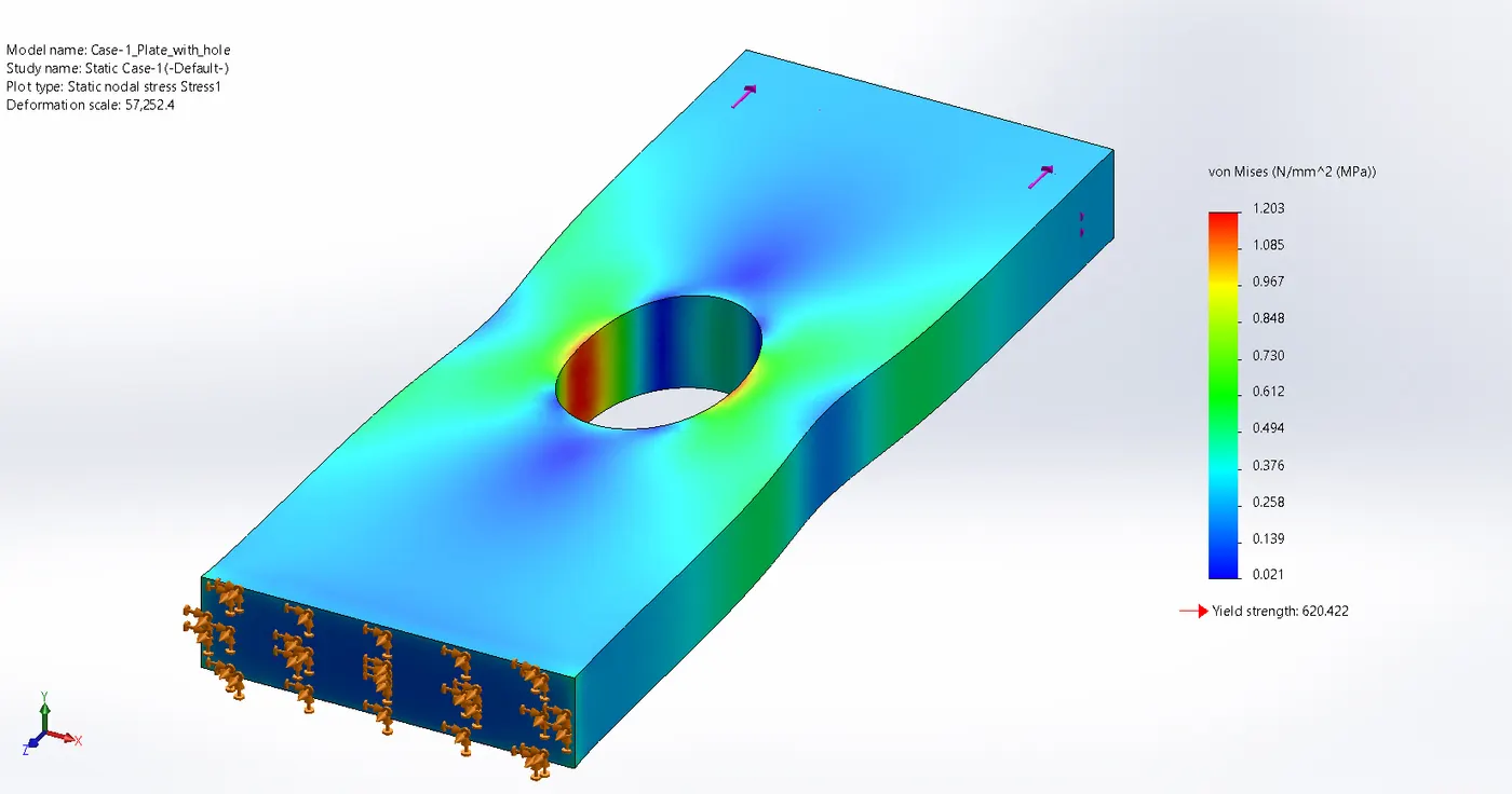
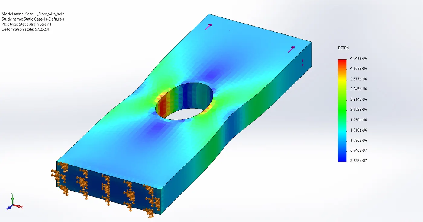
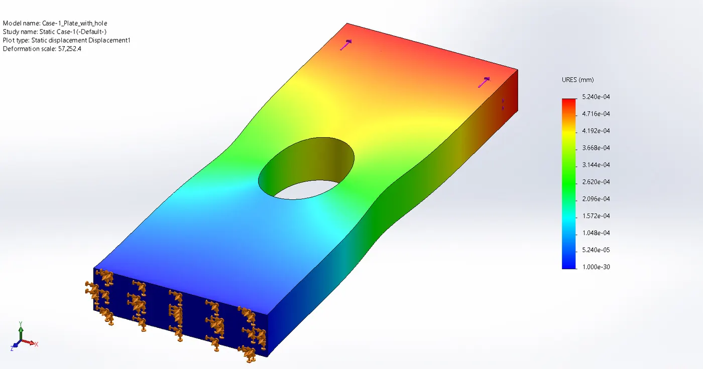
Step-4: Run the analysis and compare the results for stress, strain and displacement and output as shown below.
i. Stress:
ii. Strain:
iii. Displacement:
4.2 Case-2:
Step-1: Designing the plate with hole based on the dimension provided as shown below.
The further procedure is same as case-1 the output of this case is as follows.
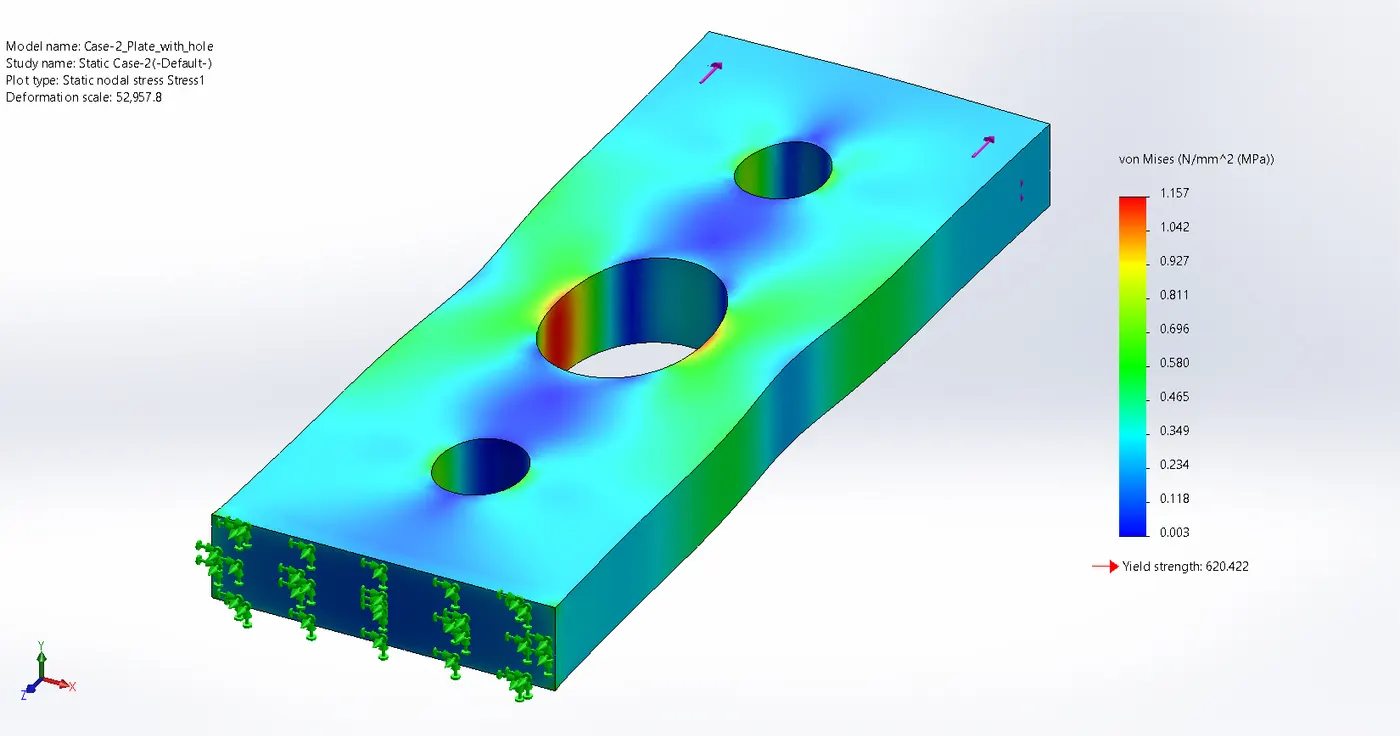
i. Stress:
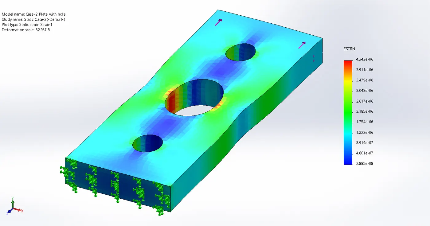
ii. Strain:
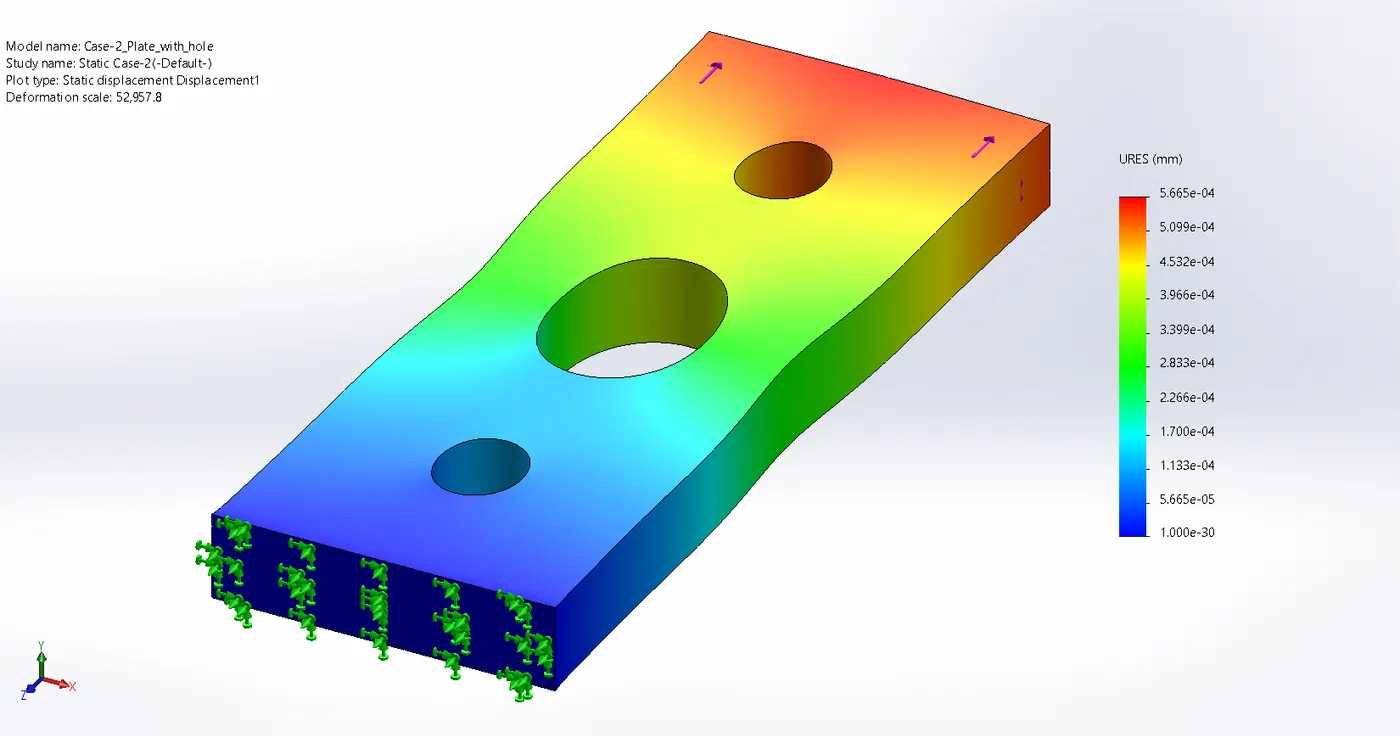
iii. Displacement:
5. Result and Conclusion:-
5.1 stress concentration varies between two geometries:
| Stress N/mm^2 | Displacement (mm) | Strain | |
| Case-1 | `1.203` | `5.240*10^(-04)` | `4.541*10^(-04)` |
| Case-2 | `1.157` | `5.665*10^(-04)` | `4.342*10^(-04)` |
Case-1 Combined Results:
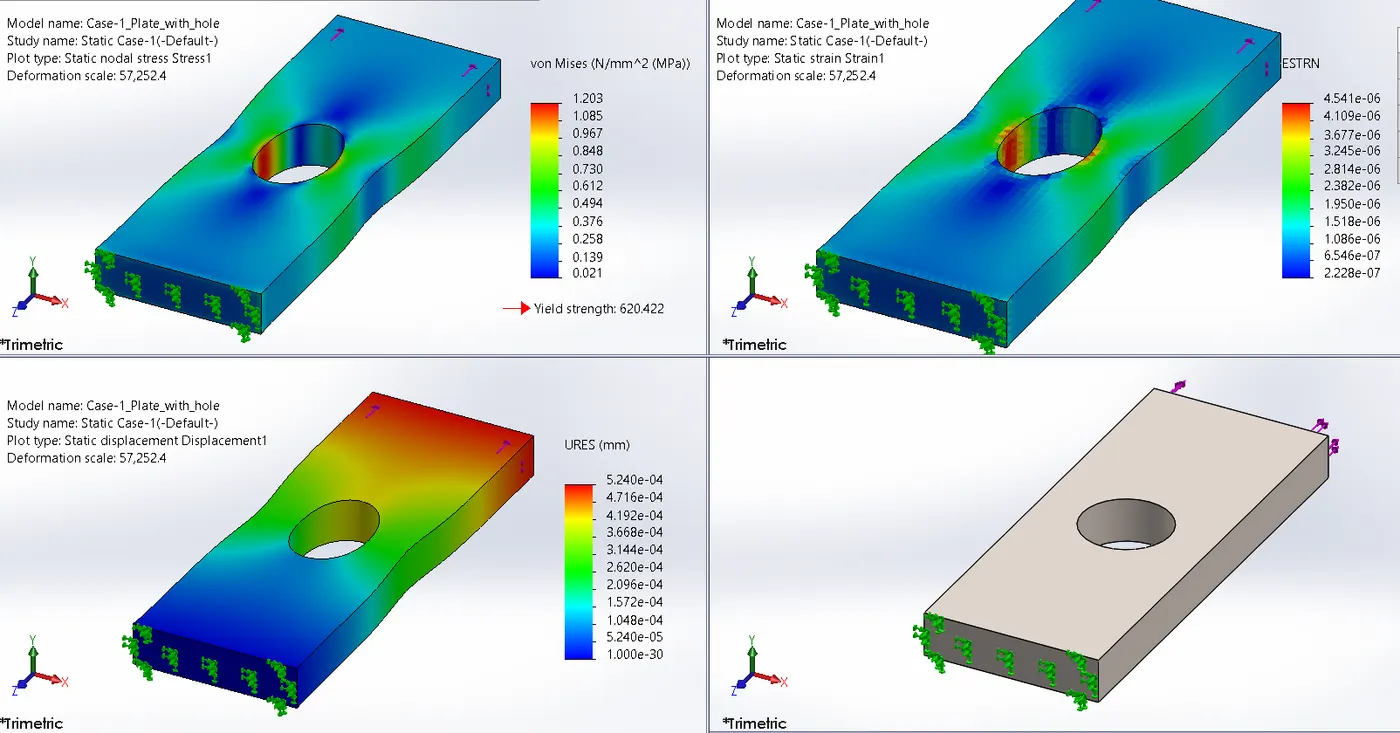
The stress concentration is uniform away from the hole and it is non-uniform in the middle of the cross-section. i.e at the hole.
Case-2 Combined Results:
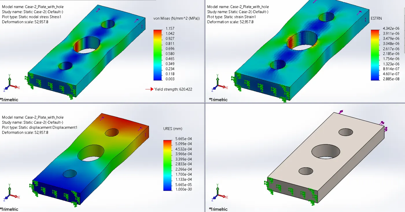
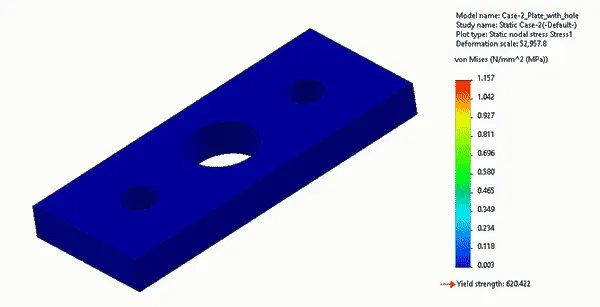
As we discussed in case-1 the stress concentration uniform away from the hole and it is non-uniform in the middle of the cross-section. i.e at the hole. the same result is applied to this also but the number of holes in increased which causes more non-uniform stress.
Stress concentrations occur at sections where the cross-sectional area suddenly changes. The more severe the change, the larger the stress concentration.
For design or analysis, it is only necessary to determine the maximum stress acting on the smallest cross-sectional area. This is done using a stress concentration factor, K, that has been determined through experiment and is only a function of the geometry of the specimen.
Normally the stress concentration in a ductile specimen that is subjected to a static loading will not have to be considered in design; however, if the material is brittle, or subjected to fatigue loadings, then stress concentrations become important.
The stress concentration factor is independent of material it's only depends upon the Geometry in many materials but for some materials the stress concentration factor is depends on the type of material also.
In a ductile material, the stress concentration is neglected because when material yields (i.e permanently deforms) it will move stress away from the stress concentration zone around the hole and forces the material around the cross-section of the hole to carry more stress. i.e the material which was holding the fewer stresses is now compensate to carry the stresses and equalized all over the material.
5.2 Validation of result:
| Cases | Parameters | Graphical Result | Analytical Result | FEA Result | Percentage Error |
| Case-1 | Maximum Stress | 1.176 Mpa | 1.1844 | 1.203 Mpa | 1.86 - 2.24 % |
| Stress concentration factor | 2.1 | 2.115 | -------------- | ||
| Case-2 | Maximum Stress | 0.95841 Mpa | 0.97156 | 1.157 Mpa | 18.544 - 19.859 % |
| Stress concentration factor | 6.9 | 6.9947 | -------------- |
Here from the above table, we can see that the percentage error in the graphical and Analytical results with respect to the FEA result is 1.86 to 2.24 % in case-1 which is very less. but in the case-2 as the holes increases in the material the stress concentration factor also increases and the percentage error, in this case, is higher as compare to the case-1. this is due to the error associated with respect to the mesh in the FEA. as we increase the number of elements in the Mesh the error will become negligible and increase in the result accuracy.
Reference:-
mechanics of materials rc hibbeler
https://mechanicalc.com/calculators/stress-concentration/
The Flow of Report:-
1. Objective.
2. Basics.
3. calculation
4. Simulation and Analysis.
5. Result and Conclusion.