CURVE FITTING USING PYTHON.
1. Objective:-
1. What do popt and pcov mean?
2. What does np.array(temperature) do?
3. What does the * in *popt mean?
4. Write code to fit a linear and cubic polynomial for the Cp data. Explain if your results are good or bad.
5. What needs to be done in order to make the curve fit perfect?
2. Curve fitting Concept:-
2.1 Basic Terms:-
Curve fits are used to describes how data changes Mathematically. This is useful for the data where formulas are not possible. even then we can get a rough trend’s by curve fitting, we can mathematically construct the functional relationship between the observed dataset and parameter values, etc.
In our problem, we are going to Plot the linear and cubic fit curves along with the raw data points. before that, we need to understand what is a linear and cubic polynomial.
i. Linear polynomial:
a linear polynomial is a polynomial of degree one. i.e the highest exponent of the variable is One.
Example:- `y=a⋅x+b`
ii. Quadratic polynomial: A quadratic polynomial is a polynomial of degree 2.
Example:- `y=a⋅x^2+b⋅x+c`
iii. Cubic polynomial:
a cubic polynomial is a polynomial of degree Three. i.e the highest exponent of the variable is Three.
Example:- `y=a⋅x^3+b⋅x^2+c⋅x+d`
2.1 Defining popt and pcov:
i. popt:- The popt argument is the best-fit parameters for Coefficients defined in the function for the curve fit. The popt holds the Coefficients (unknowns).
ii. pcov:- The pcov variable contains the covariance matrix, which indicates the uncertainties and correlations between parameters. This is most useful when the data has uncertainties.
2.2 Defining np.array(temperature):-
To give power to each element of an array or to perform any mathematical operations (like addition or subtraction) either on every element of an array or between the arrays, we need to import the numpy library. Here we called the numpy module but to use it we are using (np) because we imported the numpy module is as "import numpy as np". The temperature is an array because it contains more than one value, so we need to define it first. hence using an array(temperature) here.
2.3 Defining *popt:-
popt contains the value a, b and c and using (*) to refer this values. (i.e calling value of a,b,c)
3. Procedure & Explanation:-
Before Proceeding, we need to understand the file structure. To to that we are Opening the data file and we get two columns in which the first column contains the temperature (in K) and the second one contains specific heat (in KJ / Kmol-k). The data file is as follows.
Data File:
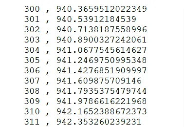
Here we can clearly see that the specific heat (Cp) which is a function of the temperature. Now, we need to fit the curve and have data set, but don’t know the mathematical formula for the curve, hence we are using the curve fit.
After observing the data we can now ready to perform curve fitting. But Before that, we need to make sure the data file is saved in the folder from where our program is going to save. This is an important step to access the data file in the program.
Step-1:- Importing Libraries.
# Importing Libraries.
import math
import matplotlib.pyplot as plt
import numpy as np
from scipy.optimize import curve_fit
Where:-
i. The "import math" and "import matplotlib.pyplot as plt" are used to use the mathematical constants and plotting the graph respectively.
ii. "import numpy as np" is used to give power to each element of an array or to perform any mathematical operations (like addition or subtraction) either on every element of an array or between the arrays.
iii. Under the scipy module, there are many inbuilt functions such as ODEINT and CURVE_FIT. Where ODEINT is basically a function which will integrate Ordinary Differential Equation (ODE) or a system of Ordinary Differential Equations and CURVE_FIT which is used in the fitting of the curve.
Step-2:- Defining Functions.
We need Code to fit a linear and cubic polynomial hence first we are defining the function for it. which is as follows.
# curve fit function for linear polynomial
def Func_Linear(t,a,b):
	return a*t+b

# Curve fit function for Cubic polynomial
def Func_Cubic(t,a,b,c,d):
return a*pow(t,3) + b*pow(t,2) + c*t + dWhere:-
The first Parameter (or) input to the curve fit function is basically a mathematical model that we are using to represent our data. i.e a*t+b for linear curve fit and a*pow(t,3) + b*pow(t,2) + c*t + d for cubic curve fit.
here we are defining a relationship between temperature and specific heat with the help of Mathematica equation. hence here we need to define the terms in the function used in the formula such as (t, a, b) for Linear curve fit and (t, a, b, c, d) for the cubic curve fit.
Step-3:- Reading Data file.
# Reading Thermodynamic Data file
def read_file():
	temperature = []
	c_p = []
	for line in open('data','r'):
		values = line.split(',')
		temperature.append(float(values[0]))
		c_p.append(float(values[1]))

return[temperature,c_p]Where:-
i. Data indicates the file name already saved in the folder where a program to be performed. 'r' indicates the mode i.e reading mode of the data file.
ii. Reading the file contents line-by-line and by using for-loop as follows.
for line in open('data','r'):
iii. we are opening a file and for each line of the file, we are running the following three command.
values = line.split(',')
temperature.append(float(values[0]))
c_p.append(float(values[1]))
Where the first line denotes the splitting line with comma operator. i.e we are using a split command to break down the line in a location where the comma exists and use arrays contains two entries such as in the first line of the data file.
iii. In Arrays the at first temperature which is indexed by [0]. similarly the second value specific heat (c_p) index by[1]. (because in python the first term (i.e Starting of data) is considered as a [0] and second as [1] and so on.
iv. The data in the data file is string value therefore we need to convert it into a float. So, to do that we are using the float command and append command used to add data in the empty arrays.
v. Return is used to return the value and save it in the empty array and till the for the for-loop executed.
Step-4:- Main Program and Plotting For a linear polynomial.
# Main Program For linear polynomial
temperature,c_p = read_file()
popt,pcov = curve_fit(Func_Linear,temperature,c_p)
fit_c_p = Func_Linear(np.array(temperature), *popt)Where:-
i. The popt argument is the best-fit parameters for Coefficients defined in the function for the curve fit. The popt holds the Coefficients (a,b,c,d, so on....).
ii. The pcov variable contains the covariance matrix, which indicates the uncertainties and correlations between parameters. This is most useful when the data has uncertainties.
iii. popt contains the value a, b and c and using (*) to refer this values. (i.e calling value of a,b,c)
# Potting linear polynomial
plt.plot(temperature,c_p,color=[0.9100,0.4100,0.1700],linewidth=2.5)
plt.plot(temperature,fit_c_p,color='g',linewidth=2.5)
plt.title('Fig.1 Specific Heat (vs) Temperature')
plt.legend(['Actual Data','Linear Curve Fit'])
plt.xlabel('Temperature (K)')
plt.ylabel('Specific Heat (kj/kmol-k)')
plt.savefig('Linear Curve Fit')
plt.show()Where:-
using the plotting command to Visualize the output result.
i. plt.plot() command is used for the plotting the actual data curve and fitted data curve.
ii. plt.title() used to provide a title to the plot.
iii. Similar to title command we can use plt.legend() command to indicate the legends in the plot.
iv We can provide a label to the plot by using plt.xlabel() and plt.ylabel() command.
v. plt.savefig() is used to save the plot as a figure in the computer.
vi. plt.show() is used to show the plots.
Step-5:-Main Program and Plotting For a Cubic polynomial..
The code and Explanation of the For a linear polynomial is applicable to this Cubic polynomial code as shown below.
# Main Program For Cubic polynomial
temperature,c_p = read_file()
popt,pcov = curve_fit(Func_Cubic,temperature,c_p)
fit_c_p = Func_Cubic(np.array(temperature), *popt)
#Plotting Cubic polynomial
plt.plot(temperature,c_p,color=[0.9100,0.4100,0.1700],linewidth=2.5)
plt.plot(temperature,fit_c_p,color='g',linewidth=2.5)
plt.title('Fig.2 Specific Heat (vs) Temperature')
plt.legend(['Actual Data','Cubic Curve Fit'])
plt.xlabel('Temperature (K)')
plt.ylabel('Specific Heat (kj/kmol-k)')
plt.savefig('Cubic Curve Fit')
plt.show()
Step-6:- Program for Best Fit.
Curve fit function for Cubic polynomial
# Curve fit function for Cubic polynomial
def Func_High(t,a,b,c,d,e,f):
	return a*pow(t,5) + b*pow(t,4) + c*pow(t,3) + d*pow(t,2) + e*t + f
Where:-
For Higher-Order Polynomial we need to define the terms in the function used in the formula such as (t, a, b, c, d, e, f).
After that, we used the same steps as discussed in the above linear and cubic Polynomial coding.
4. Final Program and Output:-
4.1 Code to fit a linear and cubic polynomial:
i. Combined Program:
# Code to fit a linear and cubic polynomial

# Importing Libraries.
import math
import matplotlib.pyplot as plt
import numpy as np
from scipy.optimize import curve_fit

# curve fit function for linear polynomial
def Func_Linear(t,a,b):
	return a*t+b

# Curve fit function for Cubic polynomial
def Func_Cubic(t,a,b,c,d):
	return a*pow(t,3) + b*pow(t,2) + c*t + d

# Reading Thermodynamic Data file
def read_file():
	temperature = []
	c_p = []
	for line in open('data','r'):
		values = line.split(',')
		temperature.append(float(values[0]))
		c_p.append(float(values[1]))

	return[temperature,c_p]


# Main Program For linear polynomial
temperature,c_p = read_file()
popt,pcov = curve_fit(Func_Linear,temperature,c_p)
fit_c_p = Func_Linear(np.array(temperature), *popt)

# For For linear polynomial
plt.plot(temperature,c_p,color=[0.9100,0.4100,0.1700],linewidth=2.5)
plt.plot(temperature,fit_c_p,color='g',linewidth=2.5)
plt.title('Fig.1 Specific Heat (vs) Temperature')
plt.legend(['Actual Data','Linear Curve Fit'])
plt.xlabel('Temperature (K)')
plt.ylabel('Specific Heat (kj/kmol-k)')
plt.savefig('Linear Curve Fit')
plt.show()

# Main Program For Cubic polynomial
temperature,c_p = read_file()
popt,pcov = curve_fit(Func_Cubic,temperature,c_p)
fit_c_p = Func_Cubic(np.array(temperature), *popt)

#For Cubic polynomial
plt.plot(temperature,c_p,color=[0.9100,0.4100,0.1700],linewidth=2.5)
plt.plot(temperature,fit_c_p,color='g',linewidth=2.5)
plt.title('Fig.2 Specific Heat (vs) Temperature')
plt.legend(['Actual Data','Cubic Curve Fit'])
plt.xlabel('Temperature (K)')
plt.ylabel('Specific Heat (kj/kmol-k)')
plt.savefig('Cubic Curve Fit')
plt.show()
ii. The output of Linear polynomial.
iii. The output of Linear polynomial.
4.2 Program for Best Fit:
i. Program:
# Code to fit a Higher order polynomial

# Importing Libraries.
import math
import matplotlib.pyplot as plt
import numpy as np
from scipy.optimize import curve_fit

# Curve fit function for Cubic polynomial
def Func_High(t,a,b,c,d,e,f):
	return a*pow(t,5) + b*pow(t,4) + c*pow(t,3) + d*pow(t,2) + e*t + f

# Reading Thermodynamic Data file
def read_file():
	temperature = []
	c_p = []

	for line in open('data','r'):
		values = line.split(',')
		temperature.append(float(values[0]))
		c_p.append(float(values[1]))

	return[temperature,c_p]

# Main Program
temperature,c_p = read_file()
popt,pcov = curve_fit(Func_High,temperature,c_p)
fit_c_p = Func_High(np.array(temperature), *popt)

plt.plot(temperature,c_p,color=[0.9100,0.4100,0.1700],linewidth=2.5)
plt.plot(temperature,fit_c_p,color='g',linewidth=2.5)
plt.title('Fig.3 Specific Heat (vs) Temperature')
plt.legend(['Actual Data','Higher Order Curve Fit'])
plt.xlabel('Temperature (K)')
plt.ylabel('Specific Heat (kj/kmol-k)')
plt.savefig('Higher Order Curve Fit')
plt.show()
ii. The output of Best Fit.
5. Result and Conclusion:-
5.1 For a linear and cubic polynomial:
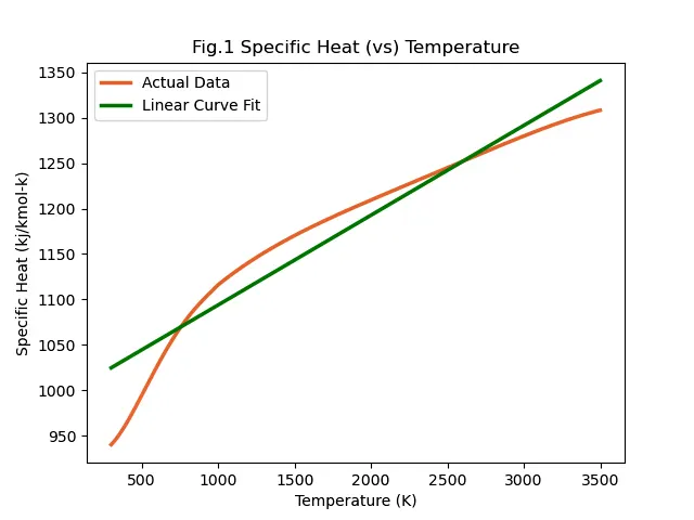
From the plot of the curve fitting with the help of linear polynomial, we can see that the path followed by the actual curve and fitted curve is in the same direction but the fitting of the curve is improper which is a bad result. Hence, the linear curve fit is not satisfied with the fitting of the curve.
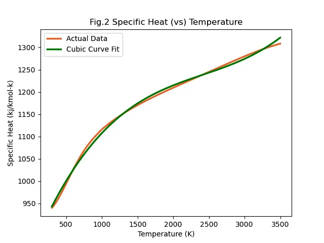
The second plot of a cubic polynomial curve follows the same direction and also a path of the actual curve with error associated with it. Hence, we can call this fit as a good fit as compared to the linear curve fit.
5.2 for Higher-Order Polynomial:
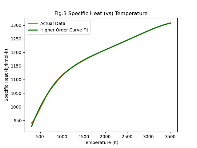
We increased the degree of polynomial which makes an actual data curve and fitted curve to follow the same path as the original. Hence, we can conclude that increasing the order of the polynomial gives us an acceptable result and Best fit out of all the cases which we did.
Though the Higher-order polynomial gives us an acceptable result, still there is an error associated with it which can be seen in the plot of a higher-order curve fit for best fit i.e fitted curve is slightly displaced from its original path at some locations during an entire plot. This indicates that we need to fit it perfectly which is as discussed below.
5.3 for the best fit:
We can conclude that to do the best fit of the curve we can increase the degree of the polynomial up to a certain limit. But to minimize the error and in order to make the curve fit perfectly, the possible solution is to Break down the temperature range into segments and perform curve fitting on each segment.
let us take an example if we have 3200 Rows and 2 columns. so to do split wise polynomial we can divide the data into 4 segments. now we get 800 data 4 times so we can apply curve fitting separately on these segments to minimise the error and to get the best possible results.
Reference:-
https://skill-lync.com/projects/Curve-Fitting-and-criterion-to-choose-best-fit-41860
https://wwwstaff.ari.uni-heidelberg.de/kruijssen/pycourse/html/15.html
https://github.com/krakjoe/pcov
The Flow Of Report:-
1. Objective.
2. Curve fitting Concept.
3. Procedure & Explanation.
4. Final Program and Output.
5. Result and Conclusion.