SIMULATE TRANSIENT BEHAVIOR OF A SIMPLE PENDULUM USING PYTHON.

1. Objective:-

i. To write a program that solves the following ODE. This ODE represents the equation of motion of a simple pendulum with damping.

`[ (d^2theta)/dt^2 + b/m*(d theta)/dt+ g/L*sin theta = 0 ]`

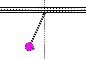
ii. Write a program in Python that will simulate the pendulum motion as shown below.

2. Basics:-

For simulating the pendulum we are using the following Ordinary Differential Equation which is Related to Standard Equation of the Mechanical Vibration to calculate the Damping and Natural Frequency of the oscillating Mechanism.
But, Here our aim to Program and find out the velocity and Displacement change of the simple pendulum concerning the time.
Hence Here we are using the Ordinary Differential Equation.

`(d^2theta)/dt^2 + b/m*(d theta)/dt+ g/L*sin theta = 0`

Where:-

b = damping coefficient in N-s/m

m = mass of the ball in kg

g = Acceleration due to gravity in m/s

L = Length in m

3. Procedure & Explanation:-

Step-1: Importing Libraries.

Before doing the program we are using the import command to import the libraries which will use for mathematical operation and plotting.

import math
import matplotlib.pyplot as plt 
import numpy as np 
from scipy.integrate import odeint

Where:-

i. The "import math" and "import matplotlib.pyplot as plt" are used to use the mathematical constants and plotting the graph respectively.

ii. "import numpy as np" is used to give power to each element of an array or to perform any mathematical operations (like addition or subtraction) either on every element of an array or between the arrays.

iii. "from scipy.integrate import odeint" command is used to do the differentiation and integration operation.

Step-2: Defining Input Parameters.

Length in m (l) = 1

Damping coefficient in N-s/m (b)= 0.05

Mass of the pendulum ball in kg (m) = 1

Acceleration due to gravity in m/s (g) = 9.81

Step-3: Initial Condition.

theta_0 = [0 ; 3]

Where first input (0) is initial Displacement and a second input (3) is an initial Velocity.

Step-4: Defining time points.

We are going to integrate the ODE system to find out the final solution, therefore we are the required value of time and as we know that, the Displacement and velocity depend on the time, hence we are defining time as follows.

t = np.linspace(0,20,150)

Where the linspace command is used to provide the initial and final value and a number of terms in between them i.e acts as a range operator. Here, the initial value is 0 and the final value is 20, and the number of values in between them is 150.

Step-5: Defining Function for Ordinary Differential Equation.

We need to solve the ODE (Ordinary Differential Equation) and plot its result. So to do that first we need to define the function based on our considered formula.
But here as we know from the basics section To write a function we need to break down the Ordinary Differential Equation.

`[ (d^2theta)/dt^2 + b/m*(d theta)/dt+ g/L*sin theta = 0 ]`

Let,

`theta = theta_1`

`(dθ_1)/dt=θ_2`

`(dθ_2)/dt=-b/m θ_2 -g/l sinθ_1`

Now to get into matrix form we we are rearranging the formula as follows.

`d/dt [[theta _1], [ theta_2]] = [[theta _2], [ -b/m θ_2 -g/l sinθ_1]]`

Let the term is as `d/dt [[theta _1], [ theta_2]] = ( d theta)/dt`

therefore the final equation becomes the funtion of `(d theta_1)/dt` and `(d theta_2)/dt`

`(d theta)/dt = (d theta_1)/dt , (d theta_2)/dt`

Using Above relationship in our function representing it as follows,

theta1 = theta[0]

theta2 = theta[1]

dtheta1_dt = theta2

dtheta2_dt = -(b/m)*theta2 - (g/l)*math.sin(theta1)

dtheta_dt = [dtheta1_dt, dtheta2_dt]

The final function is as follows:

# Function that return dz/dt
def model (theta,t,b,g,l,m):
	theta1 = theta[0]
	theta2 = theta[1]
	dtheta1_dt = theta2
	dtheta2_dt = -(b/m)*theta2 - (g/l)*math.sin(theta1)
	dtheta_dt = [dtheta1_dt, dtheta2_dt]
	return dtheta_dt

Where:- Return command is used to get multiple outputs.

Step-6: Solving ODE.

Solving ODE is nothing but calling a function which we defined above.

# Solve ODE
theta = odeint(model,theta_0,t,args = (b,g,l,m))

Where:-

odeint is a scipy module use to integrate the function to the particular time steps and keep on integrating up to the assigned value.

Step-7: Plotting.

We are plotting the graph with the help of plot command as shown below.

# Plot For Graph
plt.plot(t,theta[:,0],'g-',Label=r'$frac{dtheta1}{dt}=theta2$')
plt.plot(t,theta[:,1],'r-',Label=r'$frac{dtheta2}{dt}=-frac{b}{m}theta2-frac{g}{L}sintheta1$')
plt.xlabel('Time')
plt.ylabel('Plot')
plt.legend()
plt.title('Graph Plot')
plt.show()

Where:-

theta[:,0] represents displacement

theta[:,1] represents the velocity.

Step-8: Initial Program and Output.

Our primary program is as follows.

# Program to Solve 2nd Order ODE.

import math
import matplotlib.pyplot as plt 
import numpy as np 
from scipy.integrate import odeint

# Function that return dz/dt
def model (theta,t,b,g,l,m):
	theta1 = theta[0]
	theta2 = theta[1]
	dtheta1_dt = theta2
	dtheta2_dt = -(b/m)*theta2 - (g/l)*math.sin(theta1)
	dtheta_dt = [dtheta1_dt, dtheta2_dt]
	return dtheta_dt


# Defining Constants 
l = 1				# l = Length
b = 0.05			# b = Damping Coefficient
m = 1				# m = Mass 
g = 9.81			# g = Gravity

# Initial Condition
theta_0 = [0,3]		# Where 0 is angular displacement and 3 is angular velocity

# time points
t = np.linspace(0,20,150)

# Solve ODE
theta = odeint(model,theta_0,t,args = (b,g,l,m))

# Plot For Graph
plt.plot(t,theta[:,0],'g-',Label=r'$frac{dtheta1}{dt}=theta2$')
plt.plot(t,theta[:,1],'r-',Label=r'$frac{dtheta2}{dt}=-frac{b}{m}theta2-frac{g}{L}sintheta1$')
plt.xlabel('Time')
plt.ylabel('Plot')
plt.legend()
plt.title('Graph Plot')
plt.show()

the output of the primary program is shown below.

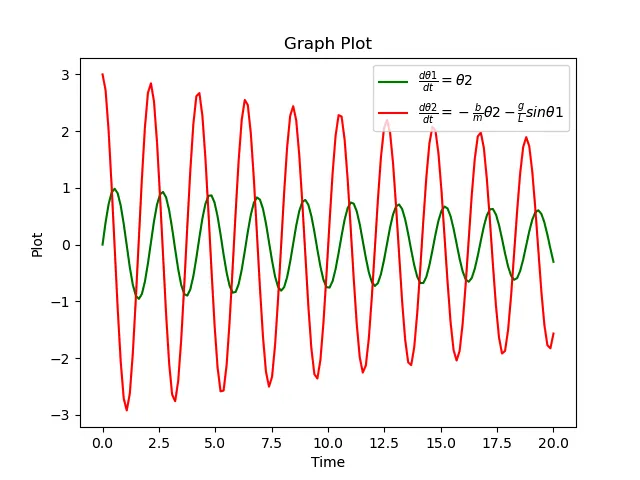
Now we get the output but we need an animated plot of the pendulum. Hence we are writing a program in the next step to get this.

Step-9: Program for Animation.

To get an animated plot of the simple pendulum we need mainly three-point to be considered as Pendulum Base, Pendulum Rope, and Pendulum Ball.

Before that, we need for-loop as,

for i in theta[:,0]:

Where We have multiple rows and 2 columns. so that (:) represents all the rows and (zero) represents the first column i.e Displacement

after that, we defined the position of the pendulum,

X0=0;
Y0=0;
x1 = l*math.sin(i)
y1 = -l*math.cos(i)

The command "filename = str(ct) + '%05d.png' % ct" is used to save the plot with the name desired name. Where ct is loop counter used to count the loop value when each time loop is get executed.

# Program For Pendulum Animation
ct=1
for i in theta[:,0]:
	x0 = 0
	y0 = 0
	x1 = l*math.sin(i)
	y1 = -l*math.cos(i)
	
	
	filename = str(ct) + '%05d.png' % ct
	ct = ct+1

	# Plot For Animation
	plt.figure()
	plt.plot([-1,1],[0,0],"black",linewidth=5) 
	plt.plot([x0,x1],[y0,y1],"black")
	plt.plot(x1,y1,'o',markersize = 30,color=[0.9100,0.4100,0.1700],markeredgecolor='black')
	plt.plot(x0,y0,'o',markersize= 6.5,markerfacecolor='w') 
	plt.xlim(-2.5,2.5)
	plt.ylim(-2.5,2.5)
	plt.title('Pendulum')
	plt.savefig(filename)

Where:-

i. [-1,1],[0,0] indicates Fix base of Pendulum

ii. x0 and y0 is the point where pendulum rope is fixed.

iii. x1, y1 Defines the position of a mass.

iv. To plot the pendulum ball, we need new commands such as markersize, markeredgecolor.

markersize:- This command used for the controlling width of the marker, just like an inline command, and to define the shape of the marker we are using 'o'. here we are using the Orange as a color but which is not predefined in the python, hence to do that we are taking the help of the internet for the code of R-G-B color combination as,
R-G-B colour combination : [0.9100 , 0.4100 , 0.1700]

V. Defining Hinge with the help of markersize, markeredgecolor command used above.

Step-10: Finalizing.

After Executing the program we are getting the 150 png files. in each file, we got a different position of the pendulum.

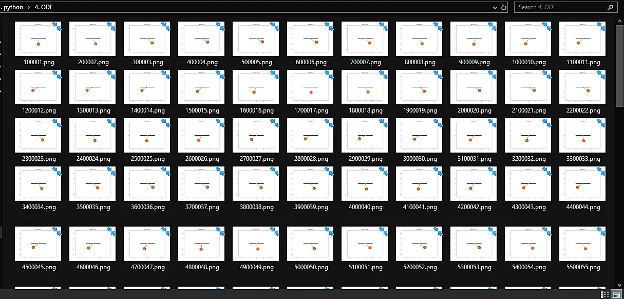
But here we need an animation, to do that we used external software and combined the image file in series and got the final pendulum animation which is shown in the result section.

4. Error & Error Elimination:-

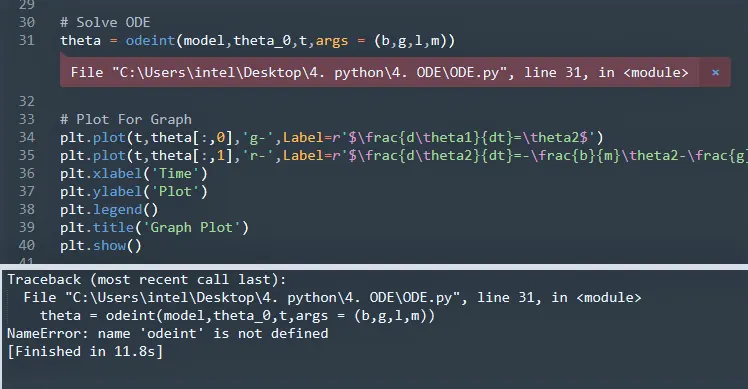
The first Error which we get is due to the improper or not imported library file for the program. Here if we have not imported the scipy module initially, we got an error as shown below.

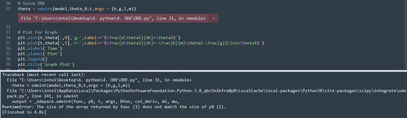
The second Error is caused due to not using the return command after the for a loop. the "return" command is used to return the value calculated in the for-loop and store it in the empty array.

5. Final Program & Output:-

# Program to Solve 2nd Order ODE.

import math
import matplotlib.pyplot as plt 
import numpy as np 
from scipy.integrate import odeint

# Function that return dz/dt
def model (theta,t,b,g,l,m):
	theta1 = theta[0]
	theta2 = theta[1]
	dtheta1_dt = theta2
	dtheta2_dt = -(b/m)*theta2 - (g/l)*math.sin(theta1)
	dtheta_dt = [dtheta1_dt, dtheta2_dt]
	return dtheta_dt


# Defining Constants 
l = 1				# l = Length
b = 0.05			# b = Damping Coefficient
m = 1				# m = Mass 
g = 9.81			# g = Gravity

# Initial Condition
theta_0 = [0,3]		# Where 0 is angular displacement and 3 is angular velocity

# time points
t = np.linspace(0,20,150)

# Solve ODE
theta = odeint(model,theta_0,t,args = (b,g,l,m))

# Plot For Graph
plt.plot(t,theta[:,0],'g-',Label=r'$frac{dtheta1}{dt}=theta2$')
plt.plot(t,theta[:,1],'r-',Label=r'$frac{dtheta2}{dt}=-frac{b}{m}theta2-frac{g}{L}sintheta1$')
plt.xlabel('Time')
plt.ylabel('Plot')
plt.legend()
plt.title('Graph Plot')
plt.show()


# Program For Pendulum Animation
ct=1
for i in theta[:,0]:
	x0 = 0
	y0 = 0
	x1 = l*math.sin(i)
	y1 = -l*math.cos(i)
	
	
	filename = str(ct) + '%05d.png' % ct
	ct = ct+1

	# Plot For Animation
	"""
	[-1,1],[0,0] indicates Fix base of Pendulum
	x0 and y0 is point where pendulum rope is fixed
	x1, y1 Defines the position of mass
	[x0,x1],[y0,y1] Defined the Rope connecting Base to the Mass

	"""
	plt.figure()
	plt.plot([-1,1],[0,0],"black",linewidth=5) 
	plt.plot([x0,x1],[y0,y1],"black")
	plt.plot(x1,y1,'o',markersize = 30,color=[0.9100,0.4100,0.1700],markeredgecolor='black')
	plt.plot(x0,y0,'o',markersize= 6.5,markerfacecolor='w') 
	plt.xlim(-2.5,2.5)
	plt.ylim(-2.5,2.5)
	plt.title('Pendulum')
	plt.savefig(filename)

The output is as below.

Conclusion:

Hence, We are able to Program to Animate simple pendulum using Python. We can take it as a reference for ODE Solver from Different types of problems.
With the help of this program and changing the data, we can use it in required applications related to the vibration problem because the simple pendulum is the representation of the spring-mass-damper system.

The flow of Report:-

1. Objective.

2. Basics.

3. Procedure & Explanation.

4. Error & Error Elimination.

5. Final Program & Output.