Analysis of Nozzle Flange of Saturn V Rocket using Ansys
1. Objective
1.1 Primary Analysis:
i. Build a nonlinear finite-element model to analyze a bolted assembly.
ii. Model contacts between parts in an assembly.
iii. Model thermal strains.
iv. Verify the finite-element model by refining the mesh and also comparing it with hand calculations.
1.2 Model Sensitivity Analysis:
i. Study the sensitivity of the bolted nozzle flange results in key input parameters as follows.
a. Load due to regeneration channels.
b. Bolt preload.
c. Coefficient of friction between flanges.
2. Introduction and Problem Specification
2.1 Introduction:
Saturn V was an American super heavy-lift launch vehicle certified for human-rating used by NASA between 1967 and 1973. it is the most powerful machine ever built. Standing at more than 100m (363ft), the Saturn V rocket burned some 20 tonnes of fuel a second at launch. Propellant accounted for 85% of its overall weight.
It consisted of three stages, each fueled by liquid propellants. It was developed to support the Apollo program for human exploration of the Moon and was later used to launch Skylab, the first American space station.
The Saturn V was launched 13 times from Kennedy Space Center with no loss of crew or payload. As of 2020, the Saturn V remains the tallest, heaviest, and most powerful (highest total impulse) rocket ever brought to operational status, and holds records for the heaviest payload launched and largest payload capacity to low Earth orbit (LEO) of 310,000 lb (140,000 kg), which included the third stage and unburned propellant needed to send the Apollo command and service module and Lunar Module to the Moon. take a look at the following awe-inspiring video below to get a sense of the tremendous power packed into this rocket.
The Saturn V consisted of three stages—the S-IC first stage, S-II second stage, and the S-IVB third stage—and the instrument unit. All three stages used liquid oxygen (LOX) as the oxidizer. The first stage used RP-1 for fuel, while the second and third stages used liquid hydrogen (LH2). Whereas LH2 has a much higher energy density to be lifted into orbit by mass, RP-1 has a much higher energy density by volume. Consequently, RP-1 was chosen for the first stage propellant because the volume of LH2 required would have been more than three times greater and would have created much higher aerodynamic drag during the boost phase through the atmosphere. The upper stages also used small solid-propellant ullage motors that helped to separate the stages during the launch and to ensure that the liquid propellants were in a proper position to be drawn into the pumps.
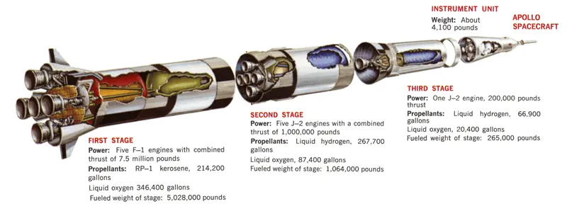
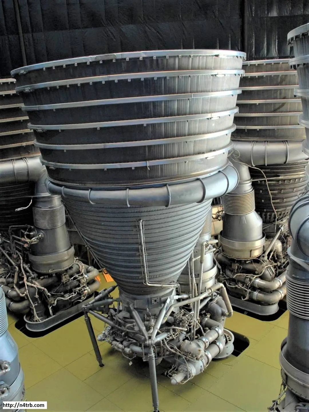
The S-IC was built by the Boeing Company at New Orleans, where the Space Shuttle external tanks would later be built by Lockheed Martin. it was powered by five Rocketdyne F-1 engines arrayed in a quincunx. The center engine was held in a fixed position, while the four outer engines could be hydraulically turned with gimbals to steer the rocket. In-flight, the center engine was turned off about 26 seconds earlier than the outboard engines to limit acceleration. During the launch, the S-IC fired its engines for 168 seconds (ignition occurred about 8.9 seconds before liftoff) and at engine cutoff, the vehicle was at an altitude of about 42 miles (67 km), was downrange about 58 miles (93 km), and was moving about 7,500 feet per second (2,300 m/s).
Our Analysis is based on the Nozzle of stage 1 used in this rocket which is discussed further. first, we need to understand the problem specification as follows.
2.2 Problem Specification:
As we know from the introduction, the Saturn V's first stage was powered by five F1 engines. In this project, we analyze the bolted flange joint that connected the mid and lower parts of the F1 engine nozzle.
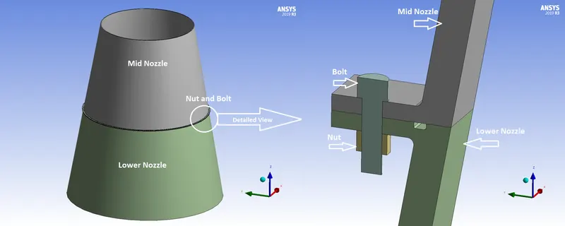
Note: The ANSYS model included in this project is shows only the mid and lower parts of the nozzle and the bolted flange joint connecting them.
We'll analyze this bolted joint by building a non-linear finite element model in ANSYS. Our main objective is to assess the margin of safety of the flange bolts. We'd also like to determine the gaps that develop between the jointed parts when the assembly is loaded.
The material properties are given in the following table:
| Material | Young's Modulus (psi) | Poisson's Ratio | Coefficient of Thermal Expansion (per deg. F) | |
| Nozzle | 300 Series Stainless Steel | 2.9E+7 | 0.27 | 1E-5 |
| Bolt and Nut | A-286 Steel | 2.9E+7 | 0.31 | 9.5E-6 |
The pressure due to the exhaust gas in the nozzle is calculated using 1D gas dynamics. It is assumed to vary linearly along the nozzle axis. The pressure at the exit (z=0) is 12.17 psi and the pressure at the entrance to the mid-nozzle is 47.72 psi.
The regeneration channels are omitted in the model. In exchange, a free body diagram is used to deduce the equivalent forces on the mid nozzle and lower nozzle (the upper nozzle is not modeled here). This force pair is modeled as two separate forces, each of 1000 lbf. The gas temperature is 700 F which causes thermal strain. We assume that the bolt is pre-loaded to 50% of its breaking strength.
3. Pre-Analysis:
Strategy:
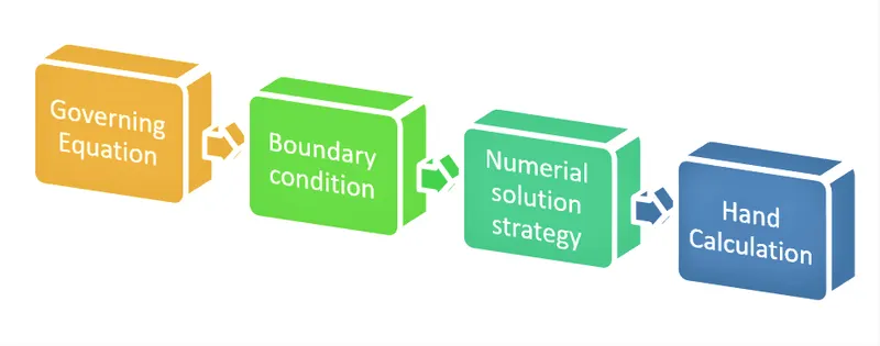
The numerical solution strategy is based on the finite-element method. i.e how the tool will solve the mathematical model. And it'll give us the displacements at the selected points, which are the nodes. our mathematical model is based on 3D elasticity. the additional complication here is that we have multiple parts rather than one part. we will see how the numerical solution strategy has to be extended to deal with that. the last element of pre-analysis is to make a hand calculation of the expected results and trends.
Domain:
The domain over which we need to solve the governing equations is given by the geometry. we model half of a bolt and nut, assuming symmetry. the model we have is with 200 bolts but we analyzing is half a bolt and the nut. it has four parts as follows on which we have to solve the governing equations of 3D elasticity over each of these parts.
a. Mid Nozzle
b. Lower Nozzle
c. Nut
d. Bolt
So, essentially we have four domains. we can think of it as having four boundary value problems that are coupled at the surfaces where we have contact or interfaces between the surfaces.
3.1. Governing Equations:
In these structural mechanics, to understand what is happening under the hood in these ANSYS, we need to know what the mathematical model is that ANSYS is solving. In particular, we need to know what are the governing equations that it's solving? What are the physical principles embedded in those governing equations? And what are the assumptions contained in the governing equations?
The governing equations are based on 3D elasticity. So here we need to take a look at the overview of what the governing equations are and the principles on which these governing equations are based which is coded into ANSYS.
3.1.1. Generalized Equation:-
These are general equations used to solve the Solid Mechanics problem which can be adjustable according to the problem requirement. Hence in our project, we see some additional equation which will be used with respect to the generalized equations which we will discuss in the next subsection "Equation for Bolted Nozzle Flange". The Generalised Equation of solid mechanics is as follows.
a. 3D Differential Equations of Equilibrium:
In the formula of 3D Differential Equations of Equilibrium, we have three equations and six unknowns.
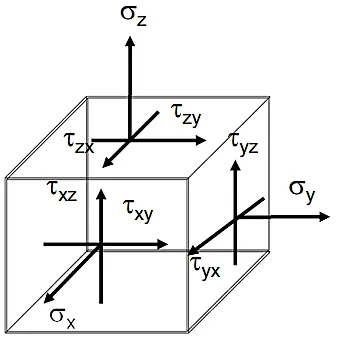
Three Equations are force balance equations in x,y, and z-direction respectively. The Six unknowns are `sigma_x, sigma_y, sigma_z, tau_(xy), tau_(xz),tau_(yz)` as shown below.
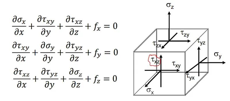
Where:-
`sigma` shows the stress in the particular direction `x,y,z` .
`tau` Shows the strain on a plane in a particular direction `x,y,z` .
`f_x,f_y,f_z = 0` which is a body force.
b. 2D and 3D Hooke's Law:
i. 2D Hooke's Law:
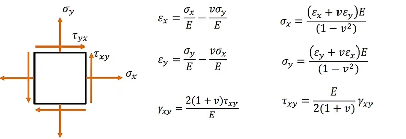
ii. 2D Hooke's Law in Matrix Form:
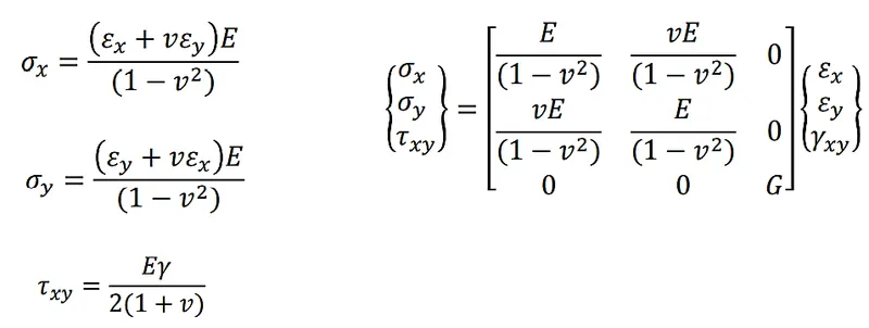
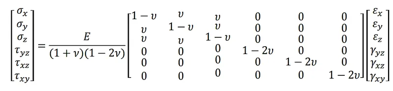
iii. 3D Hooke's Law (constructive model):
we need to bring in additional equations to close the equation set. And so we bring in the material properties through the constitutive model so that relates the stresses to the strains through the 3D version of Hooke's Law as follows.
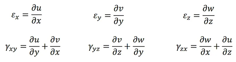
c. Strain Displacement Relation:
3.1.2. Equation for Bolted Nozzle Flange:-
As we know the governing equations are based on the equilibrium of an infinitesimal element. We have force balance in the x, y, and z directions. we get three equations but have six unknowns i.e three normal stresses and three shear stresses. The same equation is applicable to our problem as shown below.
a. 3D Differential Equation of Equilibrium: (Same as Generalized Equation)
The 3D Differential Equation of Equilibrium is the same as the generalized equation from the Bolted Nozzle flange analysis.
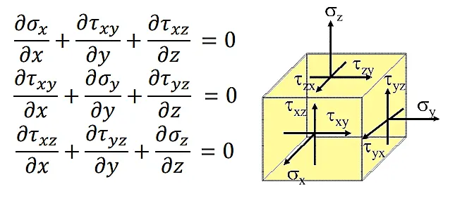
here `f_x,f_y,f_z = 0` i.e a body force is zero.
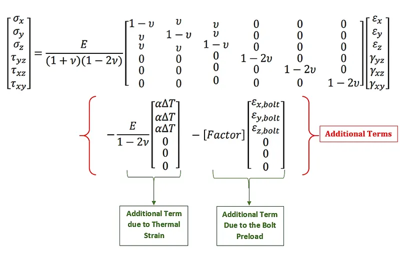
b. 3D version of Hooke's Law (constructive model):
As we discussed in the 3D version of Hooke's Law above, where we bring in the material properties through the constitutive model so that relate the stresses to the strains through the 3D version of Hooke's Law. But here we have an additional effect on the model due to the preloading of bolts and thermal strain due to hot gases as shown below.
Assumption:-
Linear Material Property i.e youngs modulus (`E`) and Poisson's ratio (`mu`) is constant. Also, the coefficient of thermal expansion (`alpha`) is not a function of temperature.
c. Strain Displacement Relation: (Same as Generalized Equation)
Note: In our Analysis, we discussed only the Main formulas. Here we are not discussed how the formula derived. To know about formulas please refer to the "Course | ENGR2000X | edX" modules 2 and 3.
3.1.3. Overall Equations and Unknowns:-
a. Equations:
3 Force balance Equation on an infinitesimal element in x,y, and z.
6 equations from a constructive model.
6 Starin Displacement Relationship.
Hence Total of 15 equations is used by Ansys to determine the Number of algebra equations.
b. Unknowns:
6 Stress components `sigma_x, sigma_y, sigma_z, tau_(xy), tau_(xz),tau_(yz)` .
6 strain components `epsi_x, epsi_y, epsi_z, gamma_(xy), gamma_(xz),gamma_(yz)` .
3 Displacement components `u,v,w` .
Hence a total of 15 unknowns is needed to find during the calculation.
Therefore we have 15 unknowns and 15 Equations which are used to solve the mathematical model.
3.2. Boundary Conditions:
Here we will review the boundary conditions that we need to put on our model. At every point on the boundary, the traction or displacement has to be defined, and this is true of normal as well as two tangential directions. So this is what we have seen before. Let's take a look at the displacement or essential boundary conditions first, and then we'll take a look at the traction or natural boundary conditions.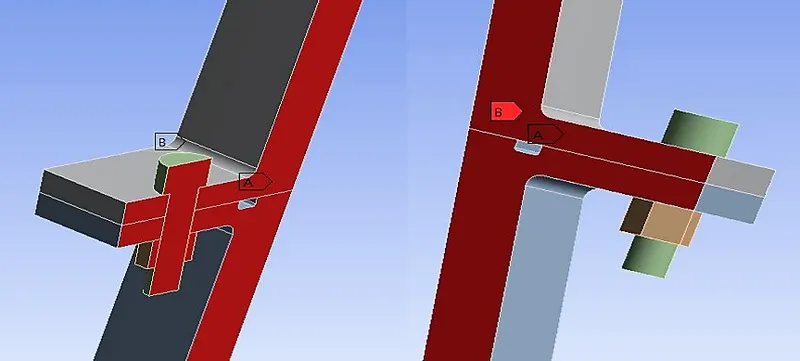
A and B show the symmetry plane. we'll get an essential boundary condition from the symmetry due to periodicity. So the symmetry surfaces, where the symmetry plane cuts the model (i.e at section A). And then the backplane is also a symmetry plane (i.e at section B).
on the symmetry plane, we basically have normal displacement is zero, and tangential traction in two perpendicular directions is zero. So it's similar to what ANSYS calls "frictionless".
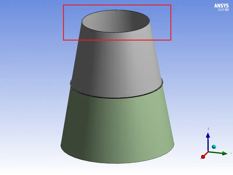
Then we also have a displacement or essential boundary condition at the top of the mid nozzle. there we have again frictionless support and "frictionless" is an ANSYS terminology. And again, the normal displacement is zero, and the tangential traction is zero. that boundary condition approximates a connection to the upper nozzle. So this part is actually connected to the upper nozzle (which we are not modeling over here).
Let's talk about traction or natural boundary conditions on the model. we have normal traction due to pressure from the propellant. So we have hot gas flowing through the nozzle, and this boundary condition models the pressure due to that. which is calculated using 1D gas dynamics.
we apply a pressure that varies in the axial direction (Z-Direction). hence it is not going to be constant pressure as shown below.
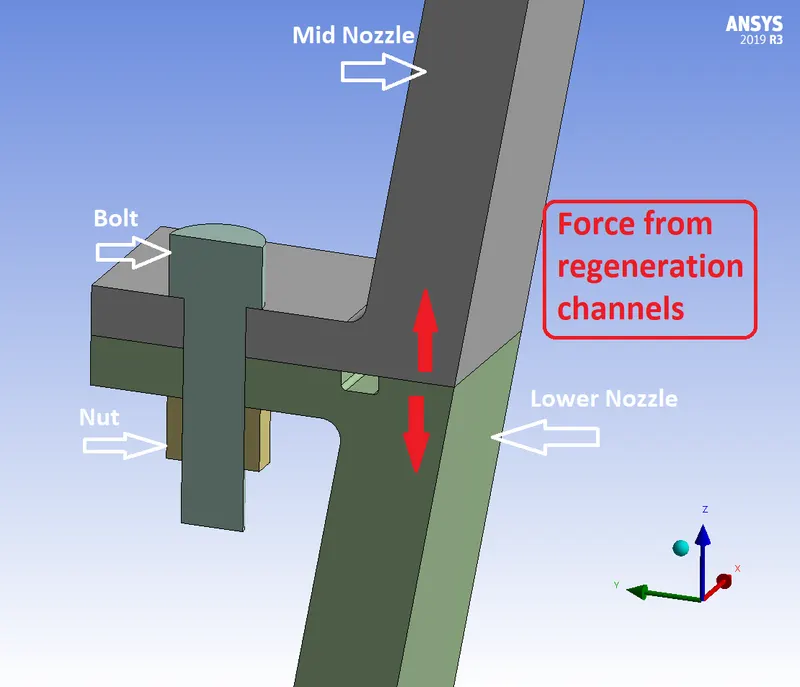
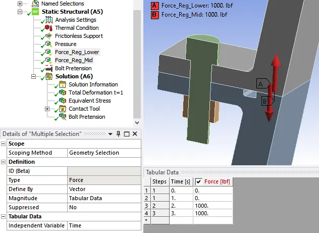
And we're also going to apply a force from the regenerative cooling channels, which, because of the pressure in those channels, which we don't model, but they tend to pull the joint apart. And those forces are modeled here. (i.e the effect is applied here in boundary condition instead of the whole model).
We won't model the channels itself, but we'll model the separation forces coming due to the pressure in those regenerative cooling channels.
Then there's also traction at the contact surfaces where the parts are going to come into contact. But we don't know a priori where the parts are going to come into contact, and that's a big complication.
And we can see that now in the deformed model, the traction on the deformed surfaces is zero because they are not in contact anymore, but where the part is in contact have traction, which means that the traction becomes dependent on the displacement.
Undeformed and Deformed Model:
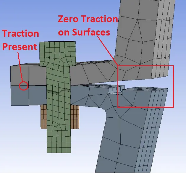
Traction at contact surfaces
– It is not known a priori where the parts are going to come into contact at the interfaces
– Traction is dependent on the displacement
i.e `overline t =overline t (u,v,w)` Which is highly nonlinear because also it can go from 0 to a finite value and so on.
3.3. Numerical Solution Strategy:
Now we want to know how that mathematical model is going to be solved and What is the strategy used in the numerical solution?
So we go from a mathematical model (boundary value problem) to a set of algebraic equations relating neighboring nodal displacements.
We have four coupled boundary value problems. we use the piecewise polynomial approximation for the three components of the displacement.
But the algebraic equations are going to be non-linear. But not all the algebraic equations are going to be nonlinear. Only the equations that are written for the nodes at the interfaces between the parts are nonlinear. because the traction becomes unknown and becomes coupled with displacement. So when we're writing the algebraic equation at the interfaces, we could get nonlinear terms, such as products of two unknown displacements.
And compare this nonlinear equation to the linear case. So we can't separate out the degree of freedom, the vector of displacements out, and multiply it by a constant matrix. we can't do that when we have nonlinear equations. So how do we need to extend this solution strategy to solve this nonlinear equation set of algebraic equations? We use the Newton-Raphson method.
So we need to find the displacement such that our set of nonlinear algebraic equations is satisfied. So if you had the exact solution to your nonlinear algebraic equations, it'll satisfy each one of those algebraic equations.
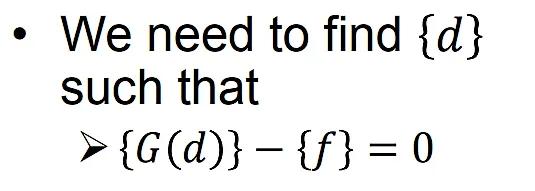
So let's say we have one nonlinear equation. And we write it in the form shown below.
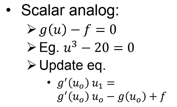
So that's a nonlinear algebraic equation above. And we want to quickly go through how to do we solve this nonlinear algebraic equation using Newton-Raphson is discussed below.
3.3.1 Newton-Raphson method ( for a single nonlinear algebraic equation.)
So here we've plotted scalar analog on the left-hand side. u on the horizontal axis. And you get some curve here. And essentially, when `g(u) - f = 0`, that's a required solution which we are looking for.
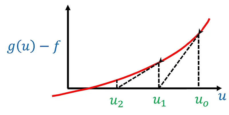
we start off with an initial guess. And then we take that initial guess and we substitute it in the equation `g(u) - f = 0`. Now, if that was the exact solution, the right-hand side would be zero. but we do not get the zero which is equal to some valve. we can interpret that as a force imbalance because of force (f).
Now we have to bring in another term to make this equal to zero. If this equation were linear, my curve would look like a slope. So we take the slope (i.e we can get the slope by differentiating the equation `g(u) - f = 0` ) further, we will use the slope to get a new guess value (u1). So we take that new guess and substitute it back in the equation `g(u) - f = 0`. Now a new equation looks like `g(u_1) - f = 0` . But we still get the imbalance which is smaller than the previous one. i.e better than the previous guess.
Now again we do the above procedure and get a better value i.e `u_2`. we can see that as we are iterating, the force imbalance is going down. But we won't get it in reality, we'll not get to the exact solution. what we can do is to check when the force imbalance is below tolerance and we will stop there. i.e the solver stops iteration when the values go below the Tolerance.
In reality, we don't have these nice smooth curves. as shown in the image above. In fact, when it comes into contact, suddenly we've gone from 0 to finite traction. So we have a nonlinear curve and there is no assurance that it's going to converge to the actual solution.
This is for a scalar equation therefore Instead of updating one value, we have to update thousands of values. So we start off with thousands of guess values, and then we keep updating that until the guess values go below the tolerance.
3.4. Hand Calculation:
Let's take a look at what kind of hand calculations one can do of the expected results. We can estimate the reaction in the axial direction with which the nozzle will be pushing on the frictionless support. We can estimate the hoop stress, that is, the circumferential stress,
and I'll get to that. We can estimate the thermal strain (input into the model)-- and the resulting deformation. that we will get to later when we apply the thermal strain into the model.
We can also do a bolt preload adjustment estimate using this particular formula, and this assumes that the flanges are infinitely rigid.
3.4.1. Axial Reaction:
We need to find the reaction in axial direction i.e z-direction. So let us take a cross-section through the nozzle, we have the pressure over the surface of the nozzle. due to this pressure, the nozzle is being pushed up, and we have frictionless support at the top so we're going to get a reaction from the frictionless support in the z-direction. The reaction will be in the negative z and we can estimate that from the pressure.
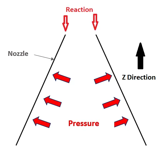
In fact, that force due to the pressure is going to be the average pressure times the projected area. taking the top radius and the bottom radius and project them. we get the two concentric circles. Now we can calculate the projected area from those two radii. And from that, we can calculate the net reaction force in the negative z-direction. So that has to balance the pressure load, which is the average pressure times the projected area.
Hence,
Average Gas Pressure:
`(12.7+47.72)/2 approx 30`
Also, Top radius is 41.75 inches and the Bottom radius is 69.50 inches.
Therefore,
The projected area in Z-direction:
`pi*r^2= pi*(69.50^2-41.75^2) = 9699` sq. inch.
Now, in our case, we have half a bolt. So we've gone from 200 bolts to half a bolt. So we have 1/400 of the model. And so, we expect our reaction in the minus z-direction to be of the order of 700 pounds as shown below.
Net reaction force in Z-direction:
`(30*9699)/400 approx 720` lbf
3.4.2. Hoop stress:
We want to estimate the hoop stress i.e circumferential stress which can be determined using the formula of hoop stress as follows.
`sigma_h = (P*D)/(2t)`
at exit p = 12.17 psi; r= 69.5 in; t = 0.5 in
hence, `sigma_h=1692` psi
4. Procedure
4.1. Geometry:
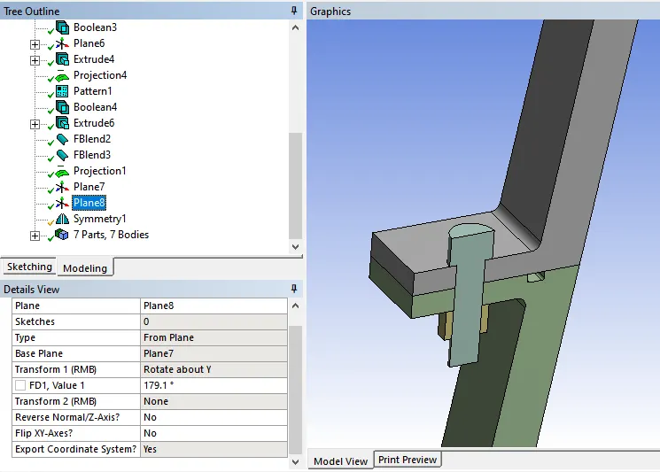
Importing Geometry to Ansys workbench under static structural Analysis. There is a boundary value problem defined by 3D elasticity, valid over each of these four parts. So we have four boundary value problems. And the four boundary value problems are coupled at the interfaces between the parts. In the tree, we can see there's a symmetrical object. This is what is used to cut the model as per periodic symmetry. we can see the symmetry planes are plane 8 and plane 7. And if we look at plane 8, we see it's offset from plane 7 by this angle of 180 degrees minus 179.1 degrees. i.e we have a 0.9-degree slice through the full model to get the reduced model, which contains half a bolt. whereas the full model contains 200 bolts.
Let us visualize full geometry first, we are going to copy the geometry in the workbench as a geometry component system. therefore dragging the geometry component in the workbench and using the default geometry by not utilizing the link between them. i.e we make a separate copy of geometry.
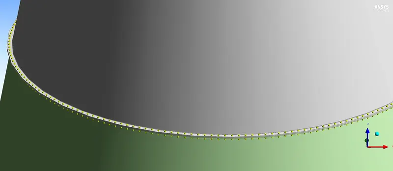
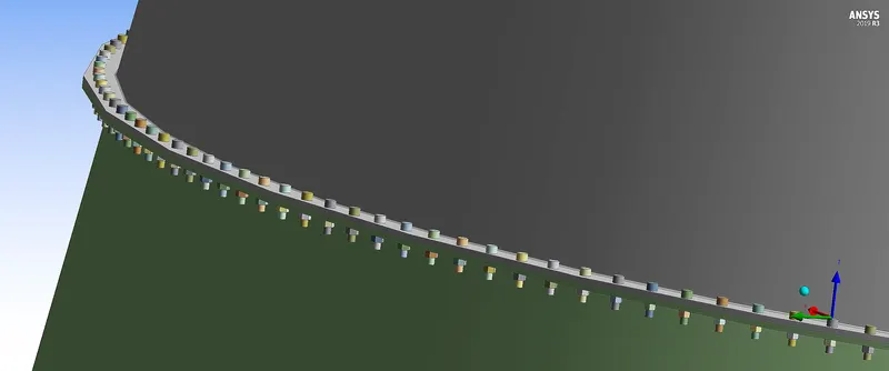
we are visualizing the geometry having half of the nut and bolt out of the 400 parts along with the mid nozzle and Lower nozzle section. i.e we have 405 parts out of which 200 is nut and 200 is bolts.
4.2. Meshing:
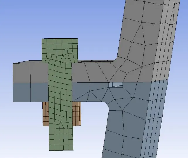
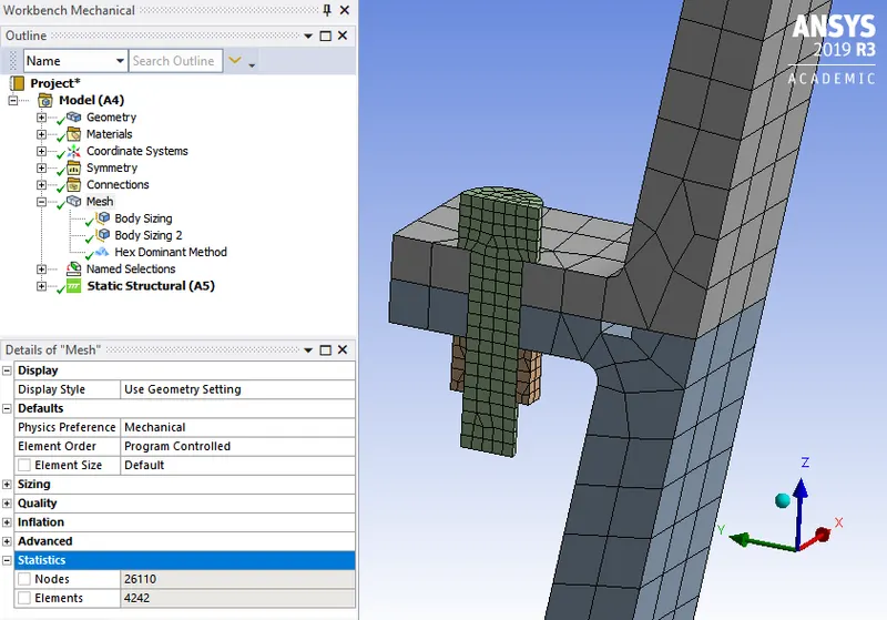
Sizing: Applying sizing for Nozzle i.e element size is 0.30 inches and for nut and bolts it is 0.075 inches. now we get a tetrahedral mesh having a number of nodes-47126 and elements-24881 we need to reduce the nodes. so we are applying the methods here.
Method: using the second-best method i.e Hex Dominant which fulfills our requirement. now our nodes are reduced to 26110.
4.2.1 Review Mesh Quality:
Let us Expand the Quality Section and select the ELement Quality option under mesh metrics. we can see it has tetrahedral, hexahedral, wedges, and pyramids. It's mostly hexahedral, but we also have other kinds. the Tet10 means that each tetrahedral element has 10 nodes, which would include the mid-side nodes. similarly the hexahedral has 20 nodes, and so on.
we can see the number of elements having a good quality mesh and few elements has poor quality mesh which affects the results. So, we need to fix that by refining the mesh. but for now, this is an acceptable mesh. So, we can go further.
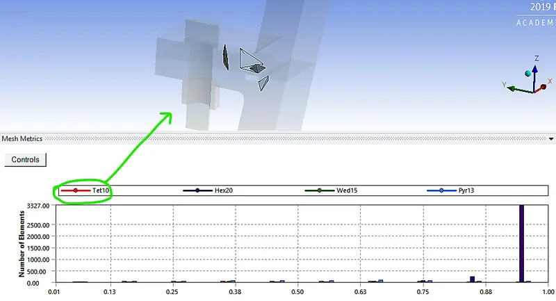
Note: we will refine the mesh while doing sensitivity analysis.
4.3. Model setup:
Because we have four domains, therefore, Ansys knows the four boundary value problem to solve. it knows to solve the 3D elasticity Equations to be solved Because we are using static structural analysis in Workbench.
In the Meshing step, we gave Ansys some key information about the numerical solution procedure. We told Ansys, what is the selected points at which we want to calculate the selected variables. Now it knows that it needs to calculate displacements because we are working on a static structural project. it also knows that the relationships between which nodes have to be written, because we have specified how the nodes are connected to form elements.
4.3.1 Specifying Material Property:
We will now specify the material properties, which we can think of specifying the constants in the governing equations. As we discussed Ansys knows that it needs to solve the 3D equations of equilibrium. the body forces are turned off by default. So there's nothing to specify here. No constants are appearing here.
where: `f_x,f_y,f_z = 0` i.e body force is zero.
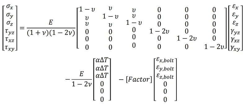
In the constitutive model, we have `E`, `mu`, and `alpha` as the three constants that we need to specify. So we'll specify that in material properties. The thermal strain and the bolt preload have not been turned on. We'll turn those on a little bit later. But we can specify alpha before that.
And in the strain-displacement relations, there are no constants appearing. So we need to specify `E`, `mu`, and `alpha` .
4.3.2 Material Property:
| Material Name | Young's Modulus | Poisson's Ratio | Coefficient of Thermal Expansion | |
| Cone | 300 series stainless steel | 2.9E7 | 0.27 | 1E-05 |
| Nut and Bolt | A-286 Steel | 2.9E7 | 0.31 | 9.5E-06 |
4.3.3 Turning on the Thermal strain:
The key point here is we are going to apply the Loads in three steps. because we have 3 types of load i.e bolt preloading, pressure, and thermal strain.

In the first load step, what we will do is we will turn on just the bolt preload. It's like, we've not loaded the model, we're just tightening the bolt. And that's going to set up some stresses in the model.
In the second load step, we are going to also apply the pressure and the forces, the separation forces, due to the regeneration channels. And that's going to affect the boundary conditions. In the second load step, we still haven't turned on the thermal effect.
In the third load step, all we do is also turn on the thermal strain. And these loads are cumulative. So at the end of the three load steps, we have the bolt preload, you have the pressure and the regeneration channel forces, and you have the thermal strain.
Now we are going to turn on load steps. to go to Ansys Mechanical >Analysis Settings > Number of steps (3 load steps).
now we are defining the thermal strain. go to Ansys Mechanical > highlight Static Structural And go to Loads > select Thermal Condition (we're going to apply the thermal strain over all the bodies.) and select Magnitude > tabular (because we want to define the magnitude in each load step).
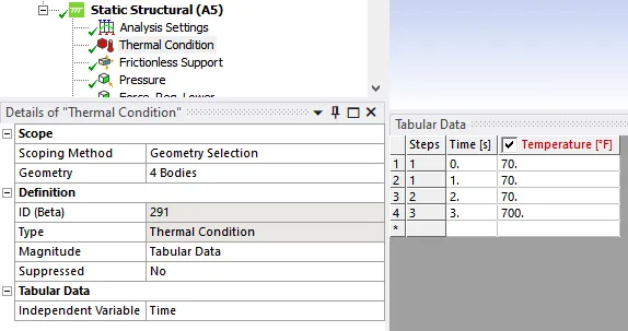
So what this table indicates. it shows at the beginning, we have everything at room temperature. And then at the end of the first load step, we still haven't turned on the thermal strain. So there's no change in temperature. At the end of the second load step, again, there's no change in temperature. And at the end of the third load step, now it's heated up to 700 degrees. So between the second and the third load steps is when the thermal strain gets turned on.
Then, at the end of the third load step, we have the full effect of the thermal strain. we have to also specify delta T, i.e change in temperature. So for that, we say the original temperature is room temperature. So go back to Static Structural and say the original temperature is just room temperature under Environmental temperature i.e 70 (degree F). So the delta T is all calculated with that as the base point.
4.3.4 Hand calculation for Thermal strain:
we know that thermal strain is `delta L= L*alpha*deltaT`
where:
`L= 160`
`alpha= 1*10^(-5)`
`deltaT=(700-70)`
therefore, `deltaL=1.008`
4.3.5 Applying the Bolt Preload:
we have given data and according to it the calculated amount of preload is 50% of the breaking strength. so to define this go to Static Structural > apply Loads > Bolt Pretension (we are going to apply it on one particular face where the threads are. And this is where it's going to feel the tension due to the preload.) And use the tabular method as we applied in thermal strain.
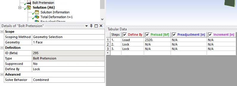
Now we are applying the 2320 pound-force. So that's applied in the first load step. And then we keep that preload on. So we say, Lock and Lock to other option. at the beginning of the first load step, this is 0. At the end of the first load step, that's applied fully. And then during the second load step, we're just going to keep that on. And the third load step, the lock means that we're going to keep that on. So that's how we're controlling that term through these settings.
4.3.6 Essential Boundary Condition:
Applying the first condition is symmetry from periodicity. And that means that surfaces can displace only parallel to itself. And there can be no displacement perpendicular to the surface.
The second condition is frictionless support at the top boundary. which means that the displacements normal to that surface have to be zero, and the tangential traction has to be zero.
4.3.7 Applying pressure and forces:
Now We will move on to specifying the traction boundary conditions. So first, we will specify the pressure due to the propellant i.e the hot gas. which is calculated using 1D gas dynamics, given data to us. So it varies in this direction. so we'll go back to Mechanical and specify that pressure. Here's Mechanical, and I will highlight Static Structural and select Loads, Pressure. And we have to select all the faces that are exposed to the hot gas Those are the inside faces of the nozzle as shown below.
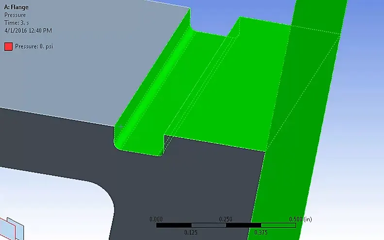
In the image above we can see that the 8 faces selected and we need to select the mid nozzle faces accordingly i.e one surface. hence we have a total of 9 faces to select.
Now apply the pressure having Magnitude which is defined by using Tabular data since I
want it to vary in the z-direction. And I'll bring the tabular data in the z-direction. And at the exit, which is z equal to 0, the pressure is 12.17 psi. then at the top, where the gas comes into the MidNozzle, we have the pressure as 47.72.
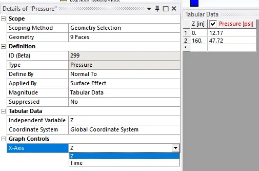
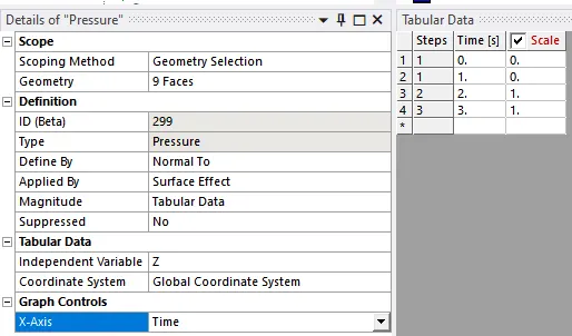
we also need to specify that this is turned on in the second load step. So I'll go to Graph Controls and change X-Axis to Time. So in the first load step, we don't apply the pressure. We just look at the effect of tightening the bolt, or the bolt pretension. And then in the second load step, it's turned on. So at the end of the second load step, the pressure is applied, it's completely applied. And then at the end of the third load step, and into the third load step, it stays on.
4.3.8 Load Due to regeneration channel:
Next, we will specify the force from the regeneration channels that are pulling apart the joint. But first, we must know how to determine the pressure due to the regeneration channel.
highlight Static Structural and say Loads, Force. And first, let's apply it to the lower nozzle. So I will select Face. And if we go to the Tabular Data, it's not turned on in the first load step. At the end of the second load step, it's 1000 pounds. And then it stays on in the third load step. similarly, we apply the load on the mid nozzle as shown below.
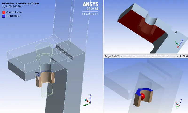
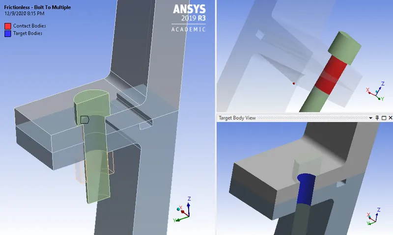
4.3.9 Specifying the contact surfaces:
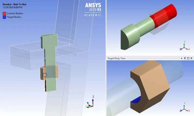
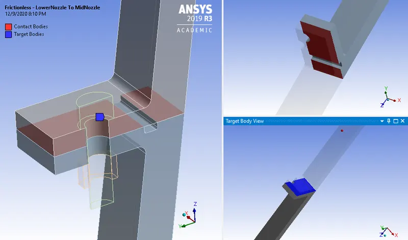
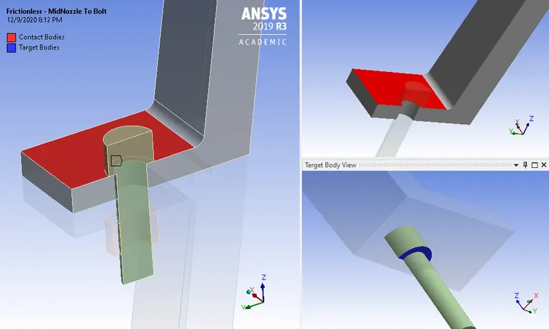
Applying the contact between the surfaces as shown below.
Bonded - Bolt To Nut:
Frictionless - LowerNozzle To MidNozzle:
Frictionless - MidNozzle To Bolt:
Frictionless - LowerNozzle To Nut:
Frictionless - Bolt To Multiple:
5. Numerical Solution
5.1. Force Convergence:
At this point, the mathematical model is completely defined, the governing equations, the domains over which we want to solve the governing equations, the boundary conditions, and the interfaces at which the domains or the parts are coupled. And we can get the ANSYS Solver to solve that mathematical model.
we have my mathematical model here and the ANSYS Solver will solve it for us by converting it to a set of algebraic equations in nodal displacements, using the piecewise polynomial approximation for u, v, and w. And there are around 27,000 nodes, and each node has 3 displacements, 3 degrees of freedom. So we have a total of around 80,000 degrees of freedom, some of which are known from the essential boundary conditions. But let's say we have around 80,000 algebraic equations to invert, some of which are nonlinear.
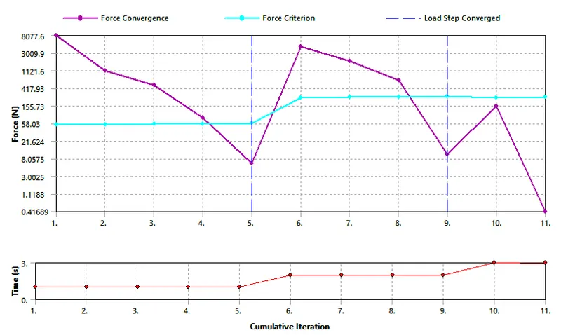
Let's get the ANSYS Solver to form those equations and invert it. go to Mechanical and highlight Solution, and say Solve. So here, it's deriving those relationships between the neighboring nodal displacements. And we can also go to the Force Convergence, which gives us a view of how the residuals from the Newton-Raphson are changing with iterations.
We also get those warnings, and if I double-click on it, it says "One or more bodies may be underconstrained and experiencing rigid body motion. Weak springs have been added." This means that it's found that the model can move. we can move in a rigid body way.
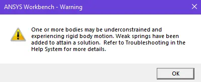
And what it did was, it picked some nodes and it constrained it and one has to make sure that that doesn't introduce kind of spurious stresses, the constraints that it's put in. One way one can do that is to look at reactions from the weak springs, and the other way is to check one's results carefully against hand calculations, which we will do further.
5.2 Plot Interpretation:
Let's talk about how to interpret the force convergence plot. let us compare with the Newton Raphson iteration. In the Newton Raphson iteration, we start off with your initial guess and update that initial guess. And if we take that value and plug it into the equation, so in this case, it won't be equal to zero. It'll be equal to some value which is an error. So that's going to be a force imbalance.
Now here, in this problem, we have around 80,000 degrees of freedom, so we have 80,000 values of force imbalance. ANSYS will give us an aggregate of those. It'll add up all those, and That's an aggregate imbalance. And it'll compare it to tolerance.
 I
I
So we can never make force imbalance to zero, but we can try to make it below some tolerance. let us discuss it step by step.
Step-1: Bolt Preloading:
In a plot, we can see that at point-1 in step-1 the imbalance is larger than tolerance so the solver updates the guess and reach point-2 in step-1 and again Got the same result but a more accurate result.
In point-5 of step-1, we can see that the imbalance is below the tolerance. Hence solver stops the calculation for step-1.
Step-2: Pressure & Regeneration force:
In step-2 the pressure is applied hence the force is increased drastically from point 5 to point-6 and which is far away from tolerance. Again guess value is updated till the guess value reaches below the tolerance i.e point 10 but here we can see that the tolerance value also increases due to an increase in the load.
Step-3: Thermal Strain:
Here we can see that the solution converges this is due to the displacements converge so much. That's meaning it may be a linearization problem that needs more iteration to confirm that. Hence Ansys iterate one more time.
6. Numerical Results and Interpretation:
Highlight Solution in the tree and first is to look at the deformation, after the first load step, after the bolt preload is applied. i.e Total Deformation at t=1. Similarly, we can add the Total Deformation at t=2 and t=3.
Then let's add the equivalent stress or von-Mises. So that gives you a single stress value for each infinitesimal element at any given location. That's kind of an amalgam of all the stress components.
We are also interested in the gap opening up between the mid nozzle and the lower nozzle between the two joined parts (because we want to make sure that there is no gas leakage). we can get the gaps by going to Tools, Contact Tool and we want to look at the gap between the lower nozzle and the mid nozzle so we will deselect all the others. And then under Contact, say Gap and again add t the gap after one-time step. i.e Gap at t=1. Similarly, we can add Gap at t=2 and t=3.
And the final object that we wanted to add Is the Bolt Pretension to Solution. So I can go ahead and say Evaluate All Results. and we will discuss the result one by one as follows.
6.1. Interpreting Deformation Results
In the model, we are plotting deformation. Now, there is deformation at different time steps. Each time step is doing something different. The very first step is preload, where we put in bolt pretension. The second is pressure, where we have our pressure loaded in the system. And the final one is we add temperature, 700 degrees. All of these are cumulative.
So we are going to take a look at time step 1. And the deformation here, we would expect that the overall flange or the overall nozzle to have very low deformation at the beginning because we're just setting the groundwork for the bolt pretension.
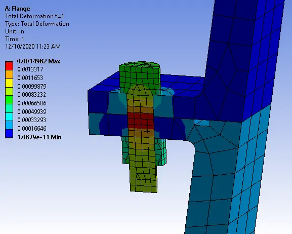
The next is the bolt pretension along with the bolt. So whenever this bolt is threaded through, there will be some deformation and movement within, and that corresponds to the preload.
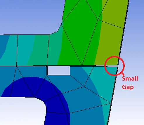
we are going to ask for total deformations at some additional time steps. therefore we are looking at the time step 2. we can see there's kind of a small gap between there. That we would expect because there is pressure trying to separate these two bodies, even though there is a bolt that's pushing them down.
Let View deformation as an Exhajurated. the fixed support at the top i.e fixed in space and the bottom of the nozzle should move out.
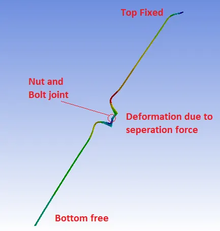
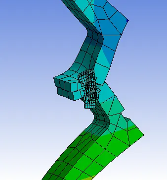
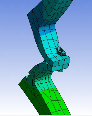
Here we're not getting as much motion from the assembly down there. And that also makes sense because we have so much material over there that it's not going to move as much. So we would expect that as well.
Similarly, we can look at the thermal step. This one is more dramatic. If we were to look at the bottom, we can see it grow axially. And again, this is the thermal time step. So it's growing radially and axially.
6.2. Interpreting Stress Results:
The bolt pretension. So my bolt pretension is 2320. The actual full bolt pretension is 4640. we divide by 2 because that's the symmetry model. But to get the stresses, I would take 2320, divide it by that cross-sectional area. And then we would obtain 60 ksi.
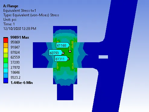
And then when it comes to the next equivalent stress stresses are, slightly higher. we are not really concerned as a stress analyst because it's designed for that.
What's interesting to us are the stresses in the nozzle? Primarily, we really want to know what's happening because of hoop stress, which is equal to the pressure
times radius over thickness. we calculated the pressure in this region is using Ansys is 12.17 psi.
When it comes to the thermal environment, the stresses don't really change. It's just that everything grows. The molecules are moving further apart based on the behavior of the atoms and molecules. However, the stresses don't change because of that. the stress is good for our result. Because I'm comparing the stresses to the capability of the material. The capability of the material for this temperature is between 15 and 20,000 psi. So stress in this region of, say, 7000 psi is well within range. We have some compressive stresses in the bolt, which is fine. We could take more look at bearing or contact stresses here and would actually see more capability. we are not too worried about that stress concentration that we saw. And then when it comes to the bolt, the bolt capability here is 160,000 psi theoretically And we're operating below 70,000 psi, indicating we have good results.
6.3 Interpreting Contact Results:
Let us look at the gap here in the preload step and this is pretty much zero. There isn't much gapping there. That's because this is the preload step, so we wouldn't really expect any gapping as shown.
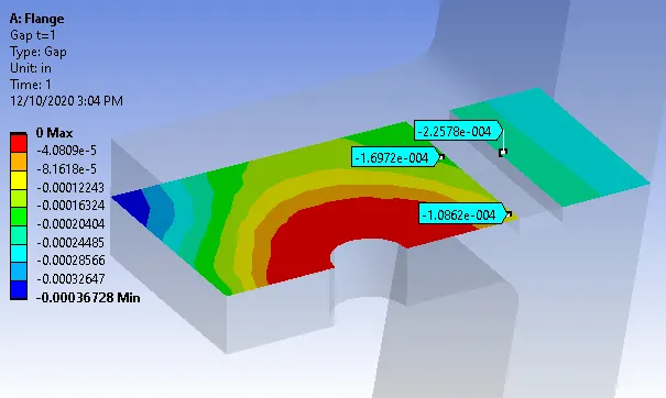
There are no outside forces that are trying to pry this thing apart. So more interesting is this second step. in the second step, the gapping over here is approximately 0.005 inches as shown below. we need more worried about the sealing agent. So that could be a metal ring or that could be an elastomer extruding through this hole. Ideally, we'd want this lower gap. Now, the gapping is effectively zero as we move away from sealing (due to the clamping).
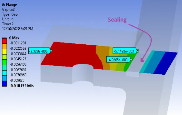
finally, In step-3 the gapping is pretty much the same as the last step. So the thermal didn't really affect it as much. Now, we would see an impact from thermal if the coefficient of thermal expansion was very different between the bolt and the actual flange material.
For example, when the body got hot, if the bolt grew more than the flange, we would expect greater gapping because we would lose some of the preload effects.
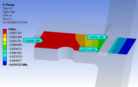
It is very difficult to predict gapping using hand calculations, so what we can do is we need to validate hoop stress and the thermal strain or the thermal growth and other areas to make sure that effects like these, which are harder to capture, are likely correct.
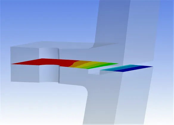
Let us view the gap more closely by increasing the gap. in general, if the gap is shown more then we need to reduce it. To reduce the gapping we can increase the preload between the bolt and nut or put in washers or a doubler between the bolt and then the flange.
6.4 Interpreting Bolt Results:
under the bolt pretension in the results, how can we look at the adjustment and what hand calculation required? how if we want to show that value in the model and then compare it to your hand calculation.
Also, When we plot the deformation in ANSYS we'll see a discontinuity in the bolt and we want to know where's that coming from?
the answer is if we were to imagine a bolt, ANSYS cuts a small delta L from that bolt. The delta L is how much material that ANSYS removes from the bolt to model the clamping to get that force. where The L represents whatever part of the bolt is modeled in ANSYS as having the preload. we are using the following formula to get that.
`deltal= (FL)/(AE)`
Where:
F = Preload
L = Length of bolt
E = Young's modulus
A = Bolt area.
Note: the preload is applied on the threaded portion of the part.
7. Verification & Validation
Here we will check how our ANSYS results compare to the hand calculations. First, let's take a look at the reaction in the axial direction and compare it to our estimate from the hand calculation.
| Hand Calculation | Ansys Result | |
| Reaction | 720lbf | 683.69 lbf |
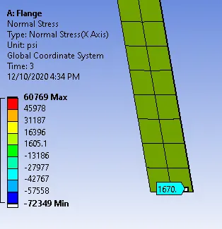
| Hoop Stress | 1692psi | 1680.2 |
| Thermal Strain | 1.008 | 1.0992 |
So the reaction is at the Frictionless Support at the top. And if I look at the results, the reaction in the x and y directions is very small, and the reaction in the z-direction is around minus 684 pounds.
And so we know we are expecting that the reaction is in the negative z-direction, so the sign matches.
And the magnitude is around 720 pound-force from the hand calculation, so that matches reasonably well.
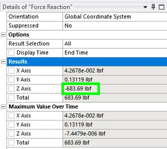
Then we had the hoop stress, and at the exit, we are expecting the value around 1,700 psi. it's the stress out of the plane, which is the x-direction. we can see it's very close to our estimate.
And the third-hand calculation that we had looked at was looking at the expansion due to the thermal strain. the total deformation is very close to our calculated value.
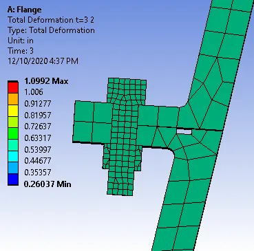
Hence we can conclude that the results are acceptable. but still, we want to do the sensitivity analysis to understand the behavior of our Model with respect to change in the parameters.
8. Sensitivity Analysis:
8.1 Changing Regeneration Channel Loads:
Let's start by doubling the load applied on both flanges by the regeneration channels. Now changing to 2,000 lbf and measuring the gap.
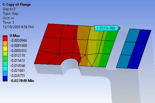
The gap increases by a factor of 3.
Explanation:
Original case: gap=−5.15∗10−3 inches
Doubled regenerative force: gap=−1.55∗10−2 inches
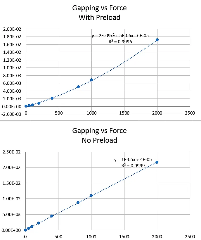
An increase in the regenerative force applied to the flanges strongly correlates with an increase in gapping. In the absence of pre-load, the flange gapping will linearly increase with load, per beam bending theory. Since pre-load is applied, the correlation between gapping and regenerative force becomes quadratic. With pre-load activated, the gapping in this case increases by a factor of 3. If pre-load was suppressed, the gap should increase by a factor of 2 (in proportion to the force increase). In application, if the gapping becomes too large, the seal (e.g. o-ring) could lodge itself in between the flanges, causing flange leaking. Thus the flange thickness, bolt choice, and seal type are functions of the regenerative force.
Here are some plots which Andy used to come to the conclusions given above. He ran the model several times to generate the data. These plots show the quadratic vs linear relationship for Gapping vs Regenerative Force.
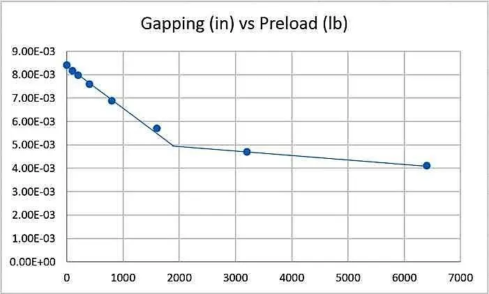
8.2 Changing Bolt Preload:
First, changing the forces applied on the flanges by the regeneration channels back to 1,000 lbf. In our base case, the bolt preload applied was 2,320 lbf. In this, let's cut that preload in half to 1,160 lbf. Leaving all other inputs the same.
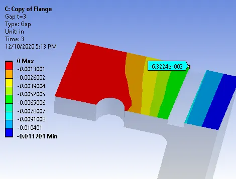
The gap increases by a factor of 1.25.
Explanation:
Original case: gap=−5.15∗10−3 inches
Halved bolt pretension: gap=−6.32∗10−3 inches
Bolt preload is a complex phenomenon and significant increases/decreases in preload do not have significant effects on the flange gap for most flange geometries. Gapping is a function of bolt and flange stiffnesses (`(AE)/L`), external loading (pressure, force), the relative thermal strain between the bolt and flange ((`(CTE_b−CTE_f)∗ΔT`), and bolt preload. Because of this, the contribution of bolt preload to gapping is influenced by the other dependent variables and may not show a simple cause and effect relationship.
Andy used the plot below to come to the above conclusions. This plot shows a roughly bilinear function for Gapping vs. Preload.
8.3 Changing to Frictional Contact:
In the base case, we modeled the contact between the two flanges as frictionless. In reality, there will be friction at the contact surfaces that will prevent them from sliding freely. To model this, change the contact between the two flanges from frictionless to frictional with a coefficient of friction = 0.5. In reality, the coefficient of friction will depend heavily on the specific material and the surface quality of the flanges.
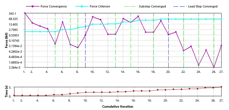
The number of iterations increased by a factor of nearly 2.5
Explanation:
Original case: 11 iterations
Frictional contact: 27 iterations
Introducing friction into the model increases the complexity of the equations to be solved and thus increases the solution time and iteration count.
Note: When we change the contact between the flanges from frictionless to frictional, the only aspect of the mathematical model that changes is the natural boundary condition at that particular contact surface.
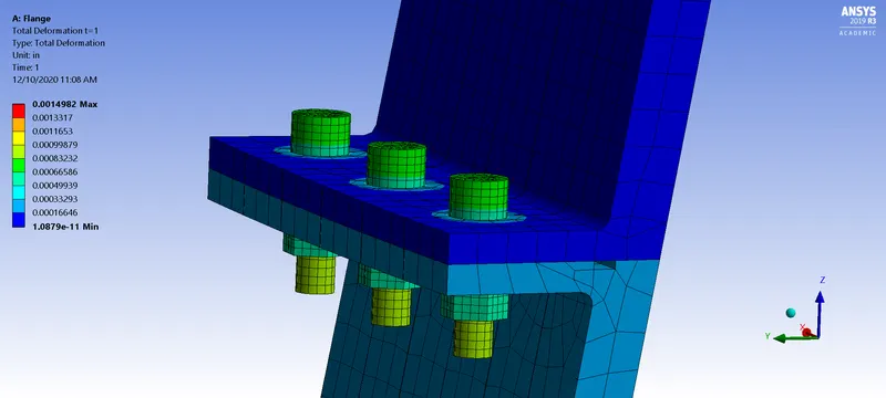
Full Nut and Bolt View:
References:
Andy Sadhwani, Aerospace Engineer SpaceX
Course | ENGR2000X | edX
Saturn V - Wikipedia
Apollo 11: Four things you may not know about the first moon landing - BBC News
How Did The Saturn 5 Rocket Work? | James May: On The Moon | Earth Lab - YouTube
The Flow of report:-
1. Objective.
2. Introduction and Problem Specification.
3. Pre Analysis.
4. Procedure.
5. Numerical Solution.
6. Numerical Result and Interpretation.
7. Verification and Validation.
8. Sensitivity Analysis.