IC ENGINE DATA ANALYSIS USING PYTHON.
1. Objective:-
-The script should take column numbers as the input and plot the respective columns as separate images.
-Each file should be saved by the name of the column.
-The plot labels should be extracted from the file. If I request for a plot between column 1 (crank angle) and column 8(volume), then the label information should automatically be extracted and must appear as labels in the plots. THIS SHOULD NOT BE DONE MANUALLY.
-Your code should exit gracefully if a non-compatible file is provided as an input. It should say something like "File not recognized. Please provide a valid CONVERGE output file".
-Calculate the area under the P-V diagram. P is in column 2 and V is in column 8.
-Calculate the power output of this engine. Assume that RPM is 1500.
-This engine consumed 20 micrograms of fuel (per 1 stroke cycle). Calculate its specific fuel consumption.
2. Basics:
File parsing refers to how to read information from a particular file (any type) and how that information can be used in a computer program. With the help of file parsing, we can access the external data and use it in our calculations. Also, with the help of file parsing, we can simplify the complex data into simple formate and we can convert data into plots to visualize it, which can be easy to understand the trend of data. Hence file parsing is also known as Task Automation. In our problem, we need to handle the data of the Internal combustion engine, therefore first we need to understand some basic terms related to the internal combustion engine which is used in our program.
2.1 Engine Terms:
i. Engine:- An engine is a machine designed to convert one form of energy into Useful work i.e Chemical energy to mechanical work. Heat engines, like the internal combustion engine, burn a fuel to create heat which is then used to do work. Electric motors convert electrical energy into mechanical motion, pneumatic motors use compressed air, and clockwork motors in wind-up toys use elastic energy. The Engine based on the conversion of Chemical energy to mechanical work is can be an internal combustion engine or external combustion engine. in our Program for the file parsing, we need to analyse the data of Internal combustion engine.
ii. Internal Combustion Engine: An internal combustion engine (ICE) is a heat engine in which the combustion of a fuel occurs with an oxidizer (usually air) in a combustion chamber that is an integral part of the working fluid flow circuit. In an internal combustion engine, the expansion of the high-temperature and high-pressure gases produced by combustion applies direct force to some component of the engine. The force is applied typically to pistons, turbine blades, rotor or a nozzle. This force moves the component over a distance, transforming chemical energy into useful work.
2.2 Performance Of ICE:-
Here We need to Plot the Pressure vs Volume diagram and also to Calculate the power output and specific fuel consumption of this engine. hence we are using the standard formula as follows.
i. The Pressure-Volume (PV) diagram: The internal combustion engine (ICE) is a heat engine. It’s working principle is based on the variation of pressure and volume inside the engine’s cylinders. All heat engines are characterized by a pressure-volume diagram, also known as PV diagram, which basically shows the variation of the pressure in the cylinder function of its volume, for a complete engine cycle.
ii. Power Output: Engine power is the power that an engine can put out. It can be expressed in power units, most commonly kilowatt, pferdestärke, or horsepower. In terms of internal combustion engines, the engine power usually describes the rated power, which is a power output that the engine can maintain over a long period of time according to a certain testing method, for example, ISO 1585. In general, though, an internal combustion engine has a power take-off shaft (the crankshaft), therefore, the rule for shaft power applies to internal combustion engines: Engine power is the product of the engine torque and the crankshaft's angular velocity. The standard formula for the power output is as follows.
`P=(2*pi*N*T)/(60*1000)(kw)`
`HP = P/0.746`
iii. Specific Fuel consumption: It is the ratio of the fuel mass flow of an engine to its output power. For reciprocating engines, it is usually given in U.S. Customary units of pound-mass per hour per horsepower [(lbm/h)/hp or lbm/(hp·h)], and International System (SI) units of kilograms per hour per kilowatt [(kg/h)/kW]. The standard formula for the specific fuel consumption is as follows.
`SFC = (mass flow rate)/(power) *3600 ((kg)/(KWh))`
3. Procedure & Explanation:-
Before Proceeding, we need to understand the file structure. To do that, we are opening the data file and Observing the file structure.
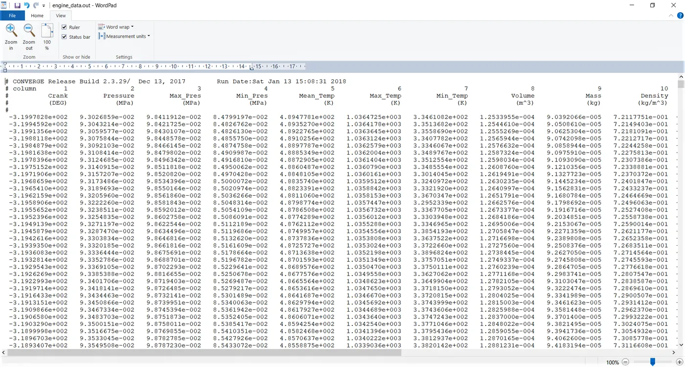
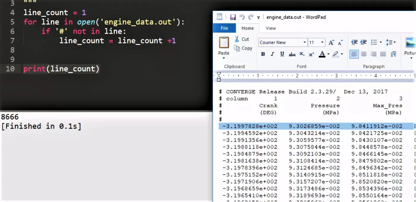
Here we can see that the data file contains multiple rows and columns containing various parameters of the engine and the total line count is 8666. hence we need to optimize it and visualise the data in the form of plot, therefore, we are using file parsing in python to get it.
Step-1: Importing Libraries.
import math
import matplotlib.pyplot as plt
import numpy as np
Where:-
i. The "import math" and "import matplotlib.pyplot as plt" are used to use the mathematical constants and plotting the graph respectively.
ii. "import numpy as np" is used to give power to each element of an array or to perform any mathematical operations (like addition or subtraction) either on every element of an array or between the arrays.
Step-2: Defining the engine parameters.
# Defining the engine parameters.

Crank = [] 			# column 1 in DEG
Pressure = [] 		# column 2 in Mpa
Max_Pres = [] 		# column 3 in Mpa
Min_Pres = [] 		# column 4 in Mpa
Mean_Temp = [] 		# column 5 in K
Max_Temp = [] 		# column 6 in K
Min_Temp = [] 		# column 7 in K
Volume = [] 		# column 8 in m^3
Mass = [] 			# column 9 in kg
Density = [] 		# column 10 in kg/m^3
Integrated_HR = [] 	# column 11 in J
HR_Rate = [] 		# column 12 in J/time
c_p = [] 			# column 13 in J/kg-K
c_v = [] 			# column 14 in J/kg-K
Kin_Visc = [] 		# column 16 in m^2/s
Dyn_Visc = [] 		# column 17 in N*s/m^2
gamma = [] 			# column 15
Where:-
Empty Array defined in each term of the engine parameters used to store the multiple values calculated.
Step-3: Compatability check.
# Compatability check
try:
	open('engine_data.out')

except:
	print('File not recognised. Please provide valid file')
Where:-
The Above Command is used due to the input data file the file satisfies the condition then it is compatible with further evaluation otherwise the error is induced as a 'File not recognised. Please provide valid file'.
Step-4: Defining the loop for Compatability check.
for line in open('engine_data.out'):
	if '#' not in line:
		Crank.append(float(line.split()[0]))
		Pressure.append(float(line.split()[1]))
		Max_Pres.append(float(line.split()[2]))
		Min_Pres.append(float(line.split()[3]))
		Mean_Temp.append(float(line.split()[4]))
		Max_Temp.append(float(line.split()[5]))
		Min_Temp.append(float(line.split()[6]))
		Volume.append(float(line.split()[7]))
		Mass.append(float(line.split()[8]))
		Density.append(float(line.split()[9]))
		Integrated_HR.append(float(line.split()[10]))
		HR_Rate.append(float(line.split()[11]))
		c_p.append(float(line.split()[12]))
		c_v.append(float(line.split()[13]))
		gamma.append(float(line.split()[14]))
		Kin_Visc.append(float(line.split()[15]))
		Dyn_Visc.append(float(line.split()[16]))
		line_count = line_count + 1
Where:-
i. For loop is used along with if condition to avoid the line containing comments and calculating multiple values and dump those values to save in the empty arrays of their respective names.
ii. Append is a command that will continuously append the value in empty arrays which we created.
iii. line_count is acted as a loop counter.
Step-6: Plotting.
# plotting
plt.grid()
plt.plot(Volume, Pressure,color='g')
plt.title('Pressure (vs) Volume ')
plt.xlabel('Volume (m^3)')
plt.ylabel('Pressure (Mpa)')
plt.savefig('Volume vs Pressure')
plt.show()

plt.grid()
plt.plot(Crank, Pressure)
plt.title('Crank (vs) Pressure')
plt.xlabel('Crank (DEG)')
plt.ylabel('Pressure (Mpa)')
plt.savefig('Crank vs Pressure')
plt.show()

plt.grid()
plt.plot(Crank, Mean_Temp,color=[0.9100,0.4100,0.1700] )
plt.title('Crank (vs) Mean Temp')
plt.xlabel('Crank (DEG)')
plt.ylabel('Mean Temp (K)')
plt.savefig('Crank vs Mean Temp')
plt.show() Where:-
using the plotting command to Visualize the output result.
i. plt.plot() command is used for the plotting the actual data curve and fitted data curve.
ii. plt.title() used to provide a title to the plot.
iii. Similar to title command we can use plt.legend() command to indicate the legends in the plot.
iv We can provide a label to the plot by using plt.xlabel() and plt.ylabel() command.
v. plt.savefig() is used to save the plot as a figure in the computer.
vi. plt.show() is used to show the plots.
Step-7: Program to calculate the Performance Parameters.
All the Above considerations and parameters are also valid for the Program to calculate the Performance Parameters hence we are not Defining it again.
# Performance calculation
# Area under P-V diagram, using column 2 & column 8.
area = np.trapz(Pressure,Volume)
print( 'Area under P-V = ',area)

# Calculating the power output of the engine by assuming RPM = 1500.
rpm = 1500 # rotations per minute
rps = 1500/60 # rotations per second
power_watt = area*rps*1000
power_hp = power_watt/0.746
print('Power output of the engine = ', power_watt)
print('Power of engine = ', power_hp)

# Calculating the Specific fuel Consumption when engine consumed 20 micro grams of fuel ( per 1 stroke cycle)
sfc = (20*pow(10,-6)*3600)/ (0.08*power_watt)
print('Specific Fuel consumption = ', sfc)
Where:-
We are using the standard formula to calculate the various parameters related to the engine as discussed in the basics.
i. since it is an iterative technique we used the trapezoidal rule for the calculation. numpy.trapz() function integrate along the given axis using the composite trapezoidal rule. np is used to perform mathematical operations.
4. Final Program and Output:-
4.1 Program for Plotting data:
i. Program:
import math
import matplotlib.pyplot as plt
import numpy as np

# Defining the engine parameters.

Crank = [] 			# column 1 in DEG
Pressure = [] 		# column 2 in Mpa
Max_Pres = [] 		# column 3 in Mpa
Min_Pres = [] 		# column 4 in Mpa
Mean_Temp = [] 		# column 5 in K
Max_Temp = [] 		# column 6 in K
Min_Temp = [] 		# column 7 in K
Volume = [] 		# column 8 in m^3
Mass = [] 			# column 9 in kg
Density = [] 		# column 10 in kg/m^3
Integrated_HR = [] 	# column 11 in J
HR_Rate = [] 		# column 12 in J/time
c_p = [] 			# column 13 in J/kg-K
c_v = [] 			# column 14 in J/kg-K
Kin_Visc = [] 		# column 16 in m^2/s
Dyn_Visc = [] 		# column 17 in N*s/m^2
gamma = [] 			# column 15

line_count = 1


# Compatability check
try:
	open('engine_data.out')

except:
	print('File not recognised. Please provide valid file')

for line in open('engine_data.out'):
	if '#' not in line:
		Crank.append(float(line.split()[0]))
		Pressure.append(float(line.split()[1]))
		Max_Pres.append(float(line.split()[2]))
		Min_Pres.append(float(line.split()[3]))
		Mean_Temp.append(float(line.split()[4]))
		Max_Temp.append(float(line.split()[5]))
		Min_Temp.append(float(line.split()[6]))
		Volume.append(float(line.split()[7]))
		Mass.append(float(line.split()[8]))
		Density.append(float(line.split()[9]))
		Integrated_HR.append(float(line.split()[10]))
		HR_Rate.append(float(line.split()[11]))
		c_p.append(float(line.split()[12]))
		c_v.append(float(line.split()[13]))
		gamma.append(float(line.split()[14]))
		Kin_Visc.append(float(line.split()[15]))
		Dyn_Visc.append(float(line.split()[16]))
		line_count = line_count + 1

# plotting
plt.grid()
plt.plot(Volume, Pressure,color='g')
plt.title('Pressure (vs) Volume ')
plt.xlabel('Volume (m^3)')
plt.ylabel('Pressure (Mpa)')
plt.savefig('Volume vs Pressure')
plt.show()

plt.grid()
plt.plot(Crank, Pressure)
plt.title('Crank (vs) Pressure')
plt.xlabel('Crank (DEG)')
plt.ylabel('Pressure (Mpa)')
plt.savefig('Crank vs Pressure')
plt.show()

plt.grid()
plt.plot(Crank, Mean_Temp,color=[0.9100,0.4100,0.1700] )
plt.title('Crank (vs) Mean Temp')
plt.xlabel('Crank (DEG)')
plt.ylabel('Mean Temp (K)')
plt.savefig('Crank vs Mean Temp')
plt.show()
ii. Output:
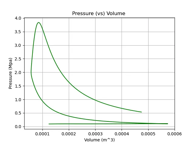
a. Pressure (vs) Volume plot.
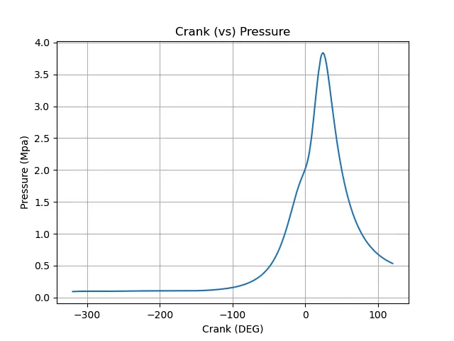
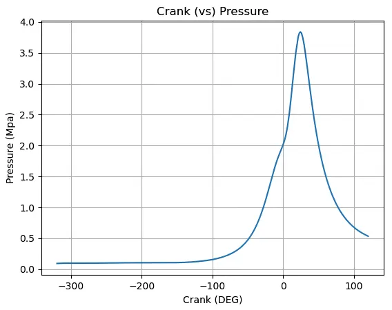
b. Crank (vs) Pressure plot.
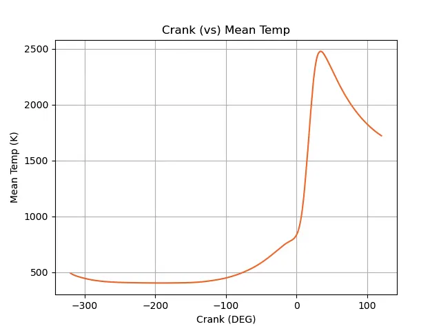
c. Crank (vs) Mean Temp plot.
4.2 Program to calculate the Performance Parameters:-
i. Program:
import math
import matplotlib.pyplot as plt
import numpy as np

# Defining engine parameters.

Crank = [] 			# column 1 in DEG
Pressure = [] 		# column 2 in Mpa
Max_Pres = [] 		# column 3 in Mpa
Min_Pres = [] 		# column 4 in Mpa
Mean_Temp = [] 		# column 5 in K
Max_Temp = [] 		# column 6 in K
Min_Temp = [] 		# column 7 in K
Volume = [] 		# column 8 in m^3
Mass = [] 			# column 9 in kg
Density = [] 		# column 10 in kg/m^3
Integrated_HR = [] 	# column 11 in J
HR_Rate = [] 		# column 12 in J/time
c_p = [] 			# column 13 in J/kg-K
c_v = [] 			# column 14 in J/kg-K
Kin_Visc = [] 		# column 16 in m^2/s
Dyn_Visc = [] 		# column 17 in N*s/m^2
gamma = [] 			# column 15

line_count = 1


# Compatability check
try:
	open('engine_data.out')

except:
	print('File not recognised. Please provide valid file')

for line in open('engine_data.out'):
	if '#' not in line:
		Crank.append(float(line.split()[0]))
		Pressure.append(float(line.split()[1]))
		Max_Pres.append(float(line.split()[2]))
		Min_Pres.append(float(line.split()[3]))
		Mean_Temp.append(float(line.split()[4]))
		Max_Temp.append(float(line.split()[5]))
		Min_Temp.append(float(line.split()[6]))
		Volume.append(float(line.split()[7]))
		Mass.append(float(line.split()[8]))
		Density.append(float(line.split()[9]))
		Integrated_HR.append(float(line.split()[10]))
		HR_Rate.append(float(line.split()[11]))
		c_p.append(float(line.split()[12]))
		c_v.append(float(line.split()[13]))
		gamma.append(float(line.split()[14]))
		Kin_Visc.append(float(line.split()[15]))
		Dyn_Visc.append(float(line.split()[16]))
		line_count = line_count + 1


# Performance calculation
# Area under P-V diagram, using column 2 & column 8.
area = np.trapz(Pressure,Volume)
print( 'Area under P-V = ',area)

# Calculating the power output of the engine by assuming RPM = 1500.
rpm = 1500 # rotations per minute
rps = 1500/60 # rotations per second
power_watt = area*rps*1000
power_hp = power_watt/0.746
print('Power output of the engine = ', power_watt)
print('Power of engine = ', power_hp)

# Calculating the Specific fuel Consumption when engine consumed 20 micro grams of fuel ( per 1 stroke cycle)
sfc = (20*pow(10,-6)*3600)/ (0.08*power_watt)
print('Specific Fuel consumption = ', sfc)
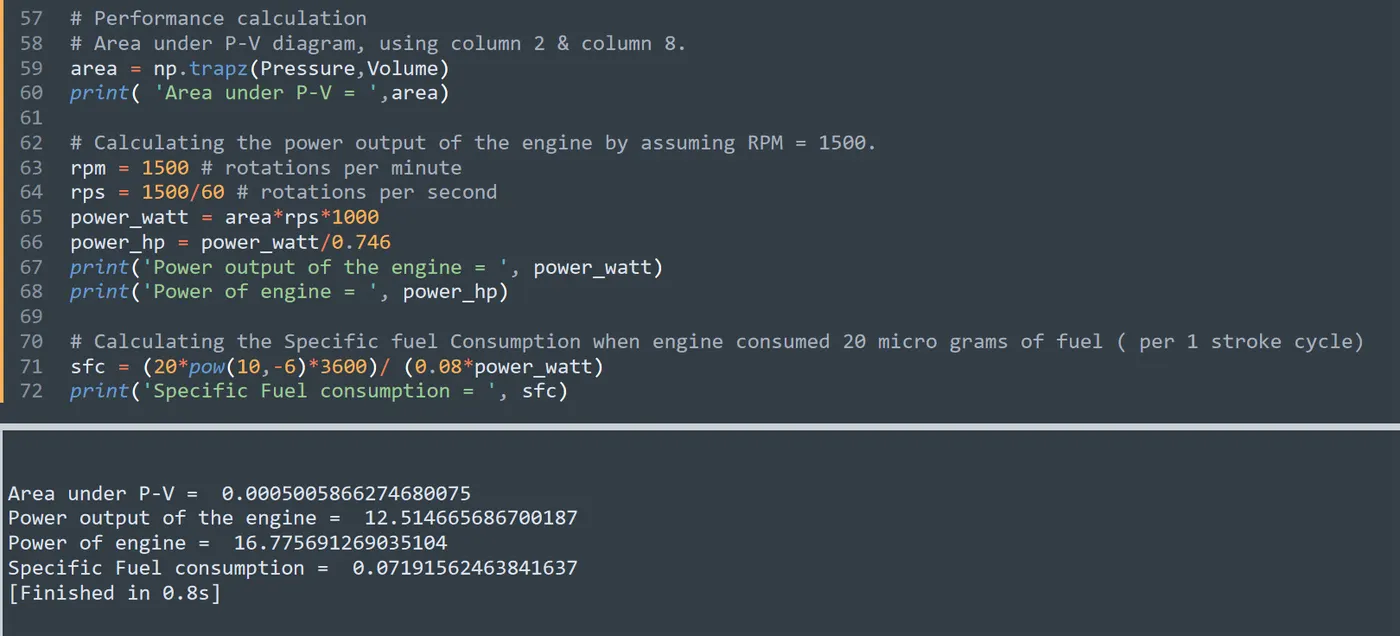
ii. Output:
5. Result and Conclusion.
From the plots, we can conclude the following results
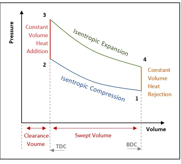
i. from the plot of the pressure-volume (PV) diagram, the changes in the volume cause the change in pressure which clearly indicates that it is a plot of an otto cycle. Hence, we can conclude that the data file of the engine_data.out is a data of Spark-ignition engine.
Where:-
1-2 Reversible Adiabatic compression (Or) Isentropic Compression.
2-3 Constant Volume Heat Addition.
3-4 Reversible Adiabatic Expansion (Or) Isentropic Expansion.
4-1 Constant Volume Heat Rejection.
Note:- Ideally the suction is neglected in the otto cycle.
A constant pressure process is represented as a horizontal line. The work done is the area under this line. If the volume is increasing through expansion, the work is done by the gas. If the arrow is reversed and the volume is decreasing, work is done on the gas.
ii. The plot of Crank (vs) Pressure and Crank (vs) Mean Temp we can conclude that the engine data file is a data of the 4-stroke Gasoline Engine (SI-Engine).
iii. The area under a PV diagram represents the work done on or by gas. Here in our case the calculated work done is 0.0005005866274680075.
iv. Also, from the main formula, we calculated the other performance parameters such as follows.
The power output of the engine in Watt= 12.514665686700187
Power of engine in HP= 16.775691269035104
Specific Fuel consumption = 0.07191562463841637
Reference:-
https://en.wikipedia.org/wiki/Engine
https://numpy.org/doc/stable/reference/generated/numpy.trapz.html
The Flow Of Report:-
1. Objective.
2. Basics.
3. Procedure & Explanation.
4. Final Program and Output.
5. Result and Conclusion.