FREQUENCY ANALYSIS OF A ROTATING SHAFT.
1. Objective:-
For this challenge, we have to find out the critical frequencies of a rotating shaft in Solidworks. we have to create the model in Solidworks.
2. Basics:-
2.1 Introduction:
Natural Frequency Analysis or Modal Analysis is carried out to understand the dynamic behavior of a system.
It helps to eliminate or reduce the vibrations caused in a component/ structure.
Vibrations are caused because of the dynamic loading and it leads to fatigue failure in a structure.
Every component/structure have their own natural frequency. When the frequency. When the excitation frequency created because the load meets the natural frequency, the system will fail.
2.2 Natural frequency analysis:
The Component/structure will deform is a shape called mode shape when the excitation frequency meets the natural frequency.
The process of calculating the natural frequency and the mode shapes is called Natural Frequency Analysis or Modal Analysis.
Rotordynamics is the part of a Modal analysis that is used to analyze the rotary systems.
2.3 Modes and Modeshape:
The mode is a shape at which the structure absorbs energy supplied by an excitation.
Mode shape depends on the geometry, constraints, and the material properties.
There are two types of modes as follows:
i. Rigid body modes.
ii.Flexible modes.
2.4 Why modal analysis?
In structural analysis, a component has to be constrained so that load applied can be counteracted by moment or reaction force. The modal analysis identifies is there any component/body needs to be constrained.
To change the mode with inconvenient frequency. The modal analysis helps us to locate where can mass be added to eliminate the failure of the component.
2.5 Types of modal analysis:
i. Unconstrained Modal Analysis:
An unconstrained component will have 6 DOF in a 3D space. If a modal analysis is carried on such type of component the first 6 mode frequency will be zero and are called rigid body modes. These modes represent the three translation and rotation of a system.
ii. Constrained Modal Analysis:
A constrained modal analysis will have Zero DOF. This analysis will have a Non-Zero value and are called as flexible modes.
If any Zero frequency mode is obtained, its source is identified and constrained.
3. Simulation and Analysis:-
3.1 Creating Model:
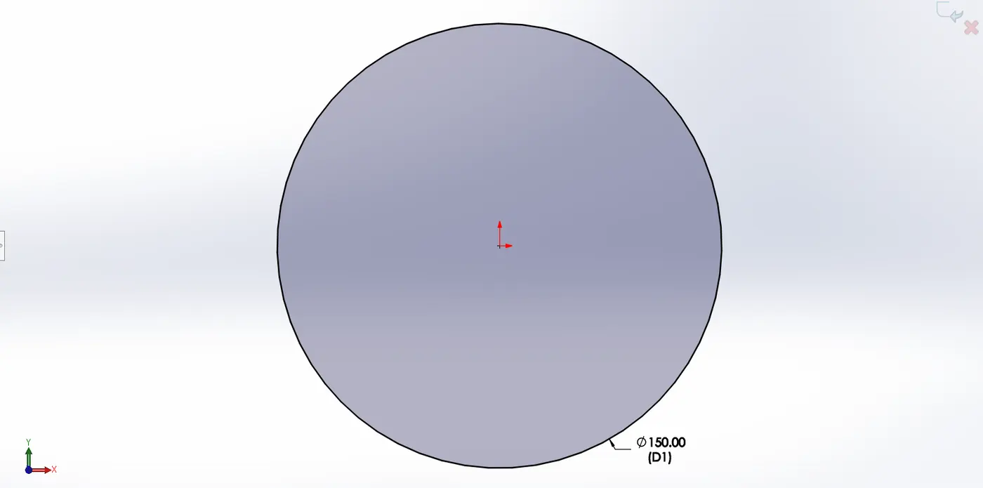
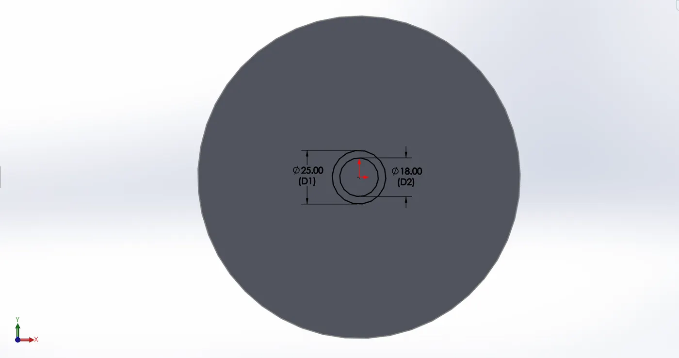
Creating the model in Solidworks based on our considered dimensions shown below.
i. Creating the main Disk.
ii. Creating Supporting Shaft.
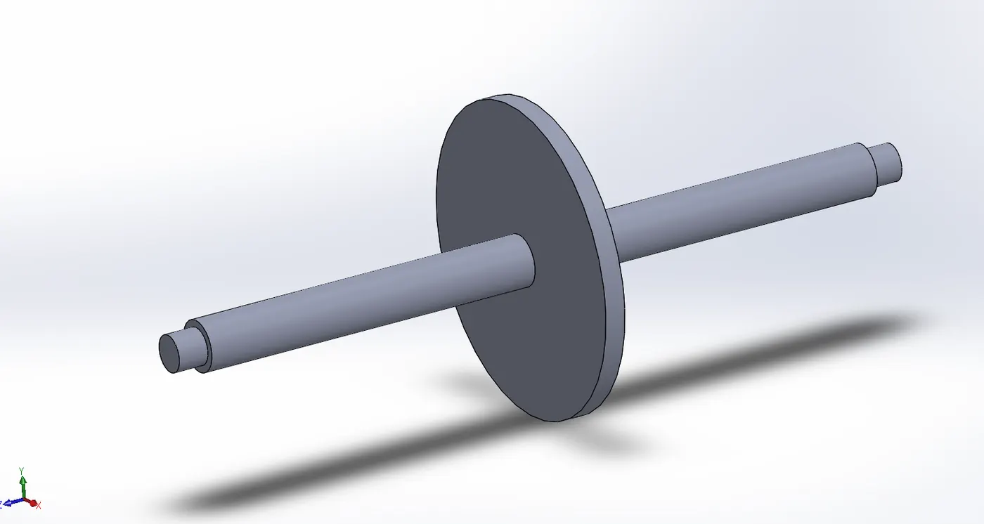
iii. After creating the disk and shaft and extending it we get our final model as shown below.
3.2 Conducting Frequency analysis :
In all the cases we have selected the alloy steel as a material which properties are given in the following table.
Material Properties:
| Property | Value | Units |
| Elastic Modulus | 210000 | N/mm^2 |
| Poisson's Ratio | 0.28 | N/A |
| Shear Modulus | 790000 | N/mm^2 |
| Mass Density | 7700 | kg/m^3 |
| Tensile Strength | 723.8256 | |
| Compressive Strength | N/mm^2 | |
| Yield Strength | 620.422 | N/mm^2 |
| Thermal Expansion Coefficient | 1.3e-05 | /K |
| Thermal Conductivity | 50 | W/(m/k) |
| Specific Heat | 460 | j/(kg.k) |
| Material Damping Ratio | N/A |
Other parameters:
| Model Type | : Linear Elastic Isotropic |
| Units | : SI-N/mm^2 (Mpa) |
| Category | : Steel |
| Name | : Alloy Steel |
| Default Failure Criterion | : Max von Mises Stress |
| Sustainability | : Defined |
Step-1: Defining the new study as frequency analysis.
Step-2: Applying material as steel defined previously.
Step-3: Applying a bearing fixture on the stepped face of the rod at the two ends to perform the analysis.
Step-4: setting Mesh to fine.
Step-5: Running simulation and output as discuss below.
3.2 Output:
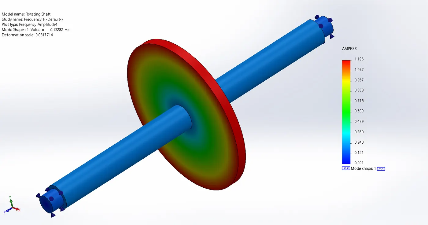
i. Mode shape-1:
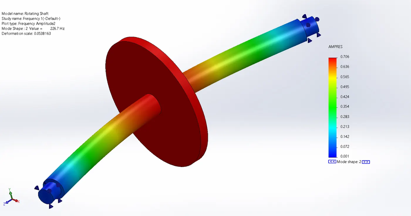
ii. Mode shape-2:
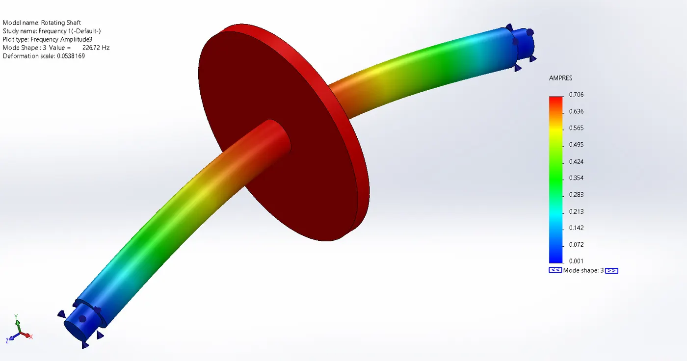
iii. Mode shape-3:
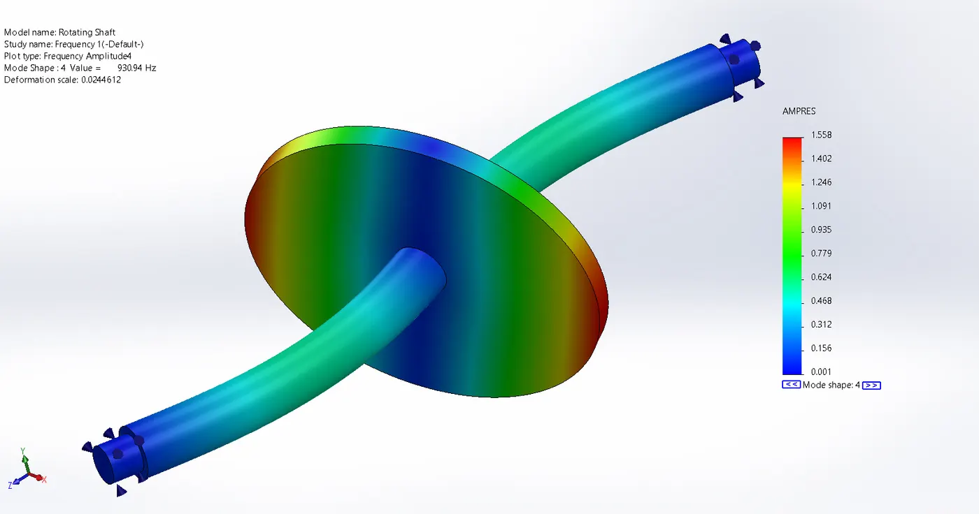
iv. Mode shape-4:
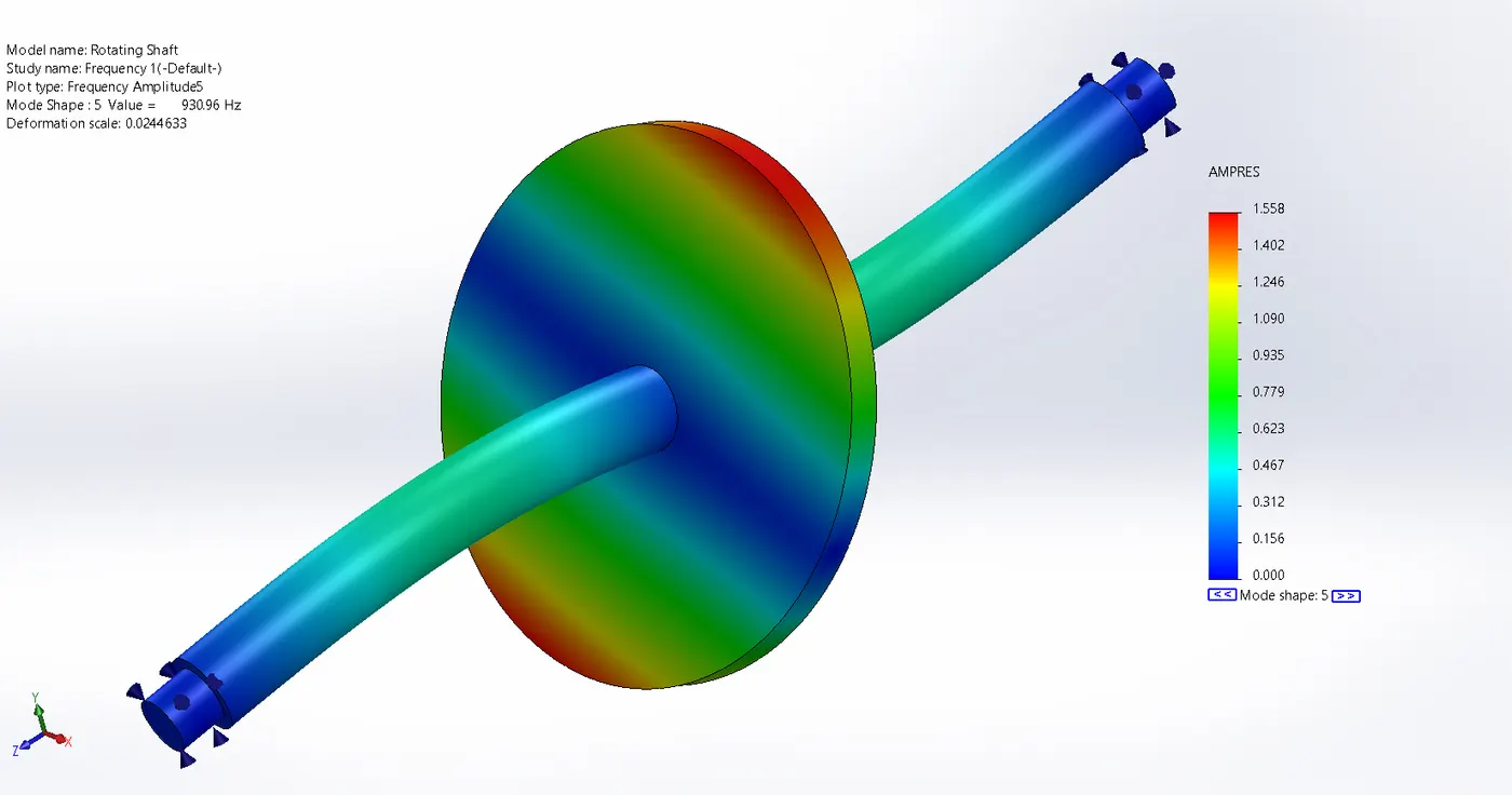
v. Mode shape-5:
4. Result and Conclusion:-
The plot of frequency mode number is as shown below
| Mode No. | Frequency(Rad/sec) | Frequency(Hertz) | Period(Seconds) |
| 1 | 0.83451 | 0.13282 | 7.5292 |
| 2 | 1424.4 | 226.7 | 0.0044111 |
| 3 | 1424.6 | 226.72 | 0.0044106 |
| 4 | 5849.3 | 930.94 | 0.0010742 |
| 5 | 5849.4 | 930.96 | 0.0010742 |
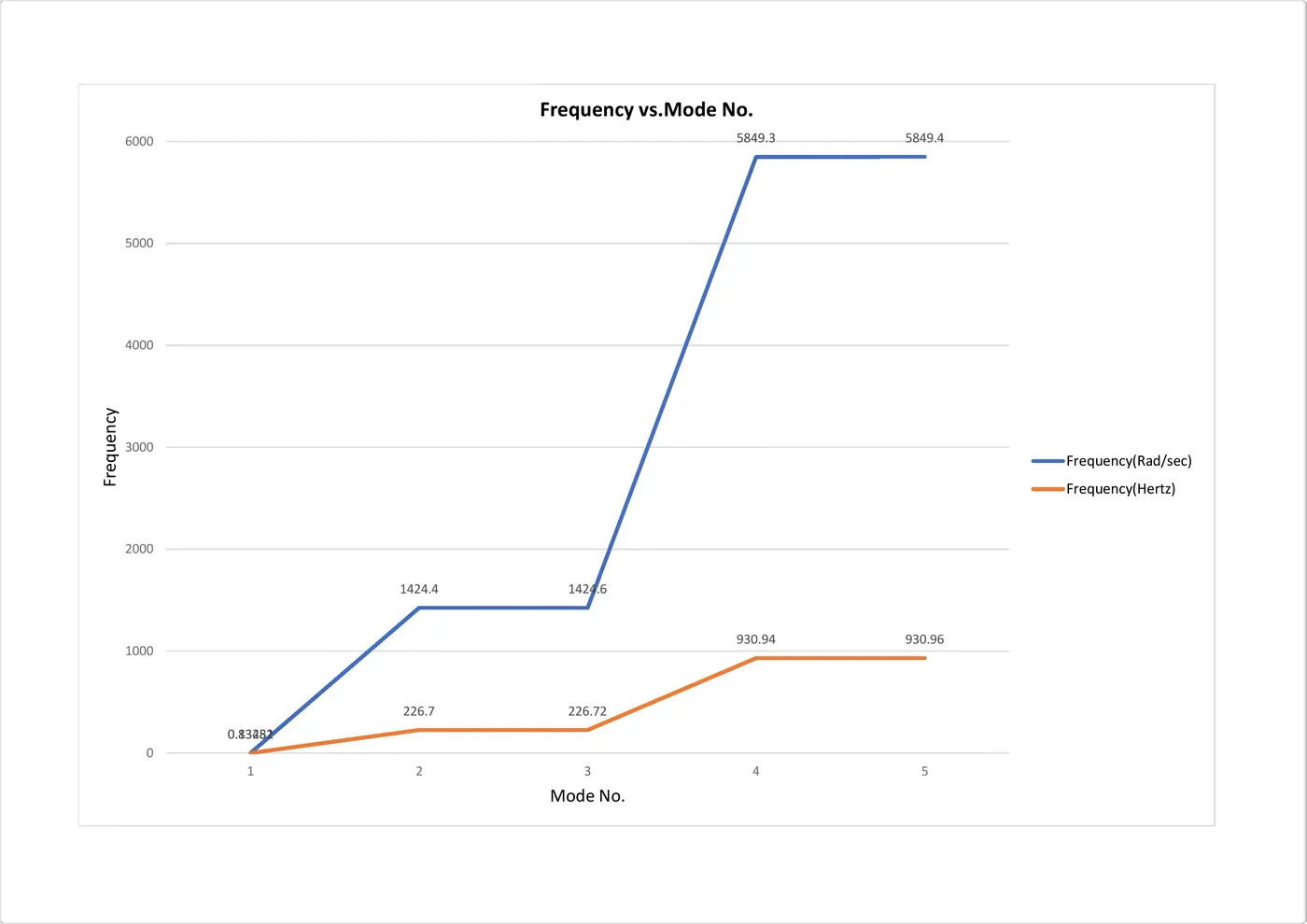
here we can see that the two frequency in which is one calculate in radian another one is calculated in the heart. i.e. it is a representation of the same frequency but in the different unit systems.
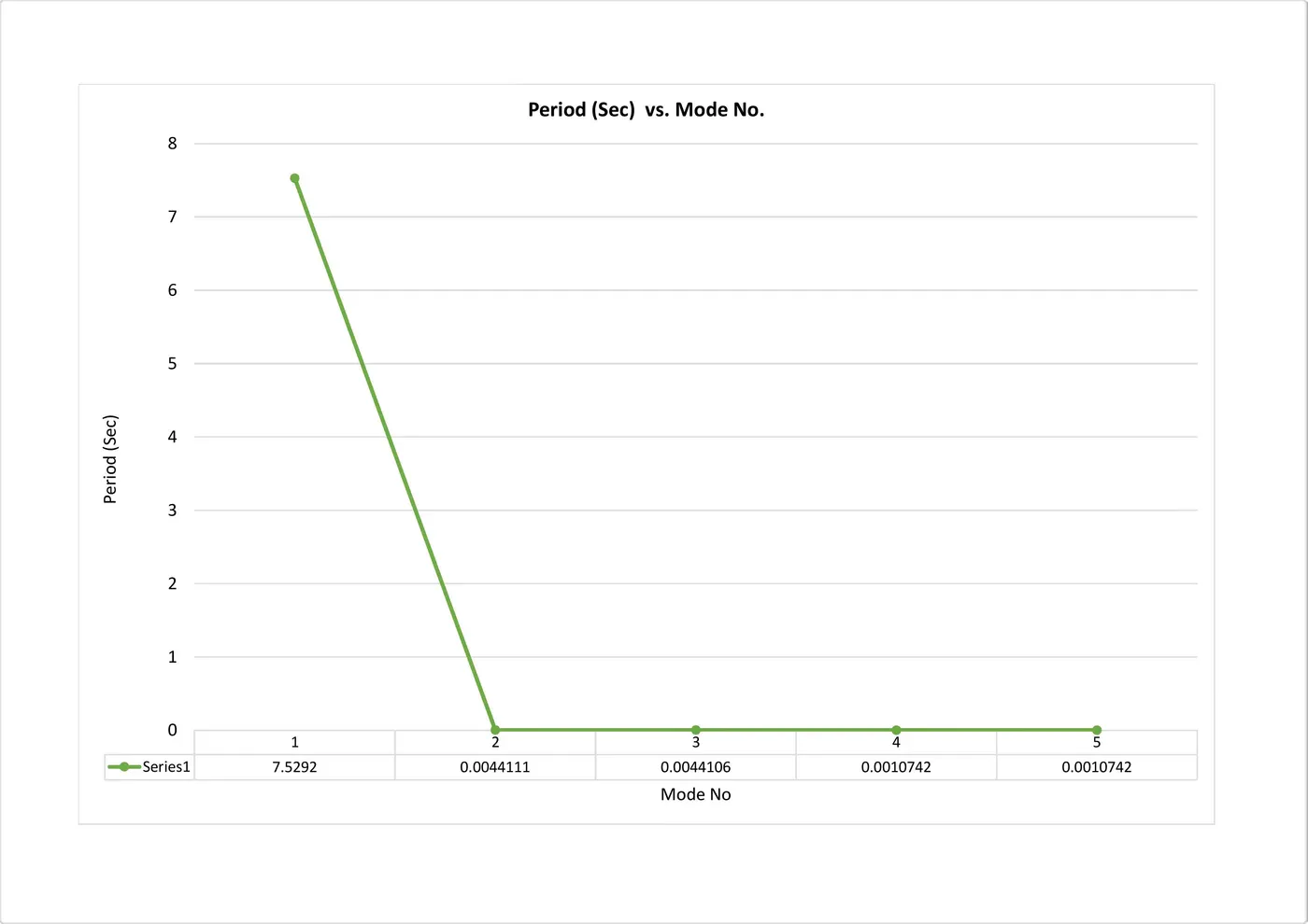
From the above plot, we can see that the variation of the period versus mode number looks linear from 2nd to 5th due to the smaller variation. Hence we are using a detail view to represent data more clear.
The detailed view of the period versus mode number is as shown below.
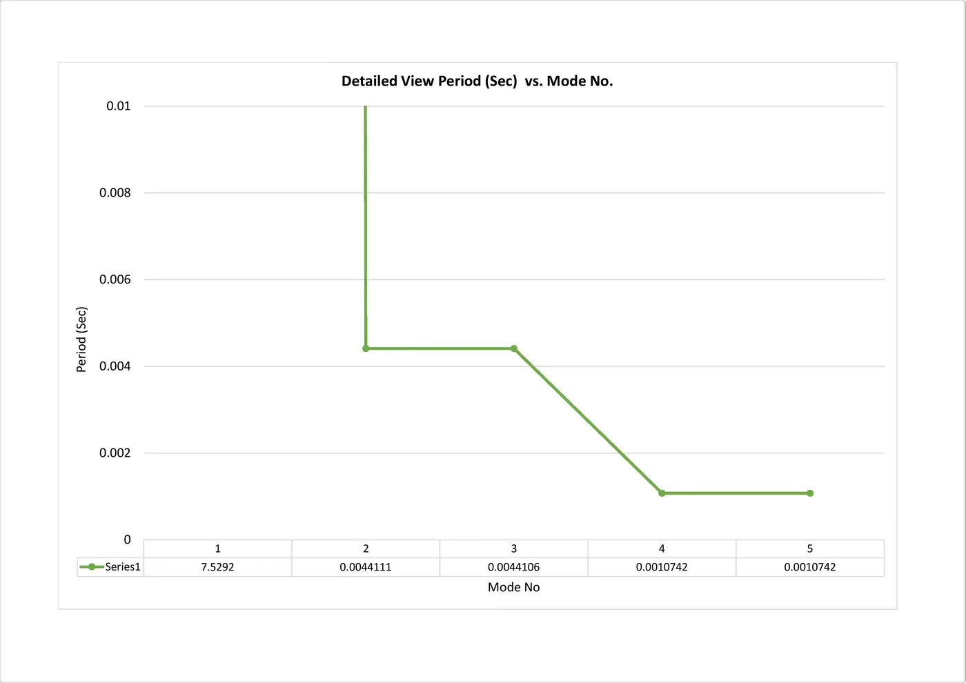
The first mode shape have frequency value near to zero because of the degree of freedom equal to 1
In the output, the resonance frequency is found. to avoid failure this resonance frequency should be considered while using this component in the machine. i.e We need to avoid the natural frequency to match while in working condition.
Reference:-
Skill-Lync Courses.
The Flow of Report:-
1. Objective.
2. Basics.
3. Simulation and Analysis.
4. Results and Conclusion.