FLOW OVER A BICYCLE
1. Objective:-
Write a Different Matlab and Python program to calculate drag force against a cyclist and get the following output.
i. plot Velocity vs Drag force.
ii. plot Drag Co-efficient vs Drag force.
2. Basic:-
2.1 Concept of Drag Force:
In general, Drag is a Resistive force exerted by the Fluid medium on the Moving Body. i.e when the body is moving in any medium then it experiences opposition force on it, which is known as Drag Force.
In case of flow over the Bicycle, a cycle area is constant but as the cyclist changes its position on the cycle it causes a change in the area. Hence Drag coefficient changes and the drag force is varying according to it.
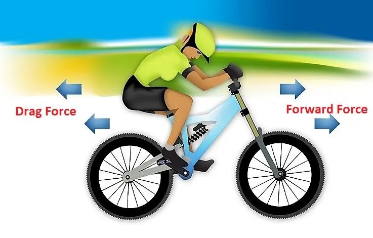
Drag force can act in different ways such as Either Fluid is moving and the body is stationary (or) Body is moving and fluid is stationary. Similarly, we can take the 3rd case where fluid and Body both move relative to each other. To calculate the Drag force we are using the standard formula as follows.
`Fd = Cd*(rho*A*V^2)/2`
Where:-
Fd = Drag force (N)
Cd = Coefficient of Drag (unitless)
ρ = Density of air (kg/m^3)
V= velocity (m/s)
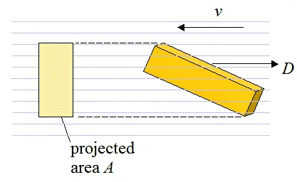
A = the projected cross-sectional area of the body perpendicular to the flow direction (that is, perpendicular to v) as illustrated in the figure below.
3. Considered Parameters:-
3.1 Parameters Considered to Calculate Drag force against a cyclist:-
In our Problem, the Fluid medium is Air and Body (or) moving object is the cyclist with a cycle, in which air is opposing the motion of cyclist. So, we can take it as a 3rd case into consideration discussed. Hence Drag force is induced. To calculate the Drag force act on the cyclist we are using the standard formula as above and the terms considered as follows
i. Drag force (Fd):- In our Problem, we are taken two Drag forces for calculating and plotting, due to the following reason.
a. To plot 'Velocity (vs) Drag force' we need variable velocity and other parameters Constant, therefore we took also Drag Co-efficient as a constant along with other constant parameters.
b. Similarly, to plot Drag 'Co-efficient (vs) Drag force' we need Variable Drag force and other parameters Constant, therefore we took also velocity as a constant along with other constant parameters.
Consideration:
In Matlab, Drag_force1 is represented as F_D1 and Drag_force2 which is represented as F_D2.
In Python, the first drag force is represented as drag_forces_1, and the second drag force is represented as drag_forces_2.
ii. Coefficient of Drag (Cd):-
In Matlab, Constant Drag Coefficient C_d1 is 0.81, and Variable Drag Coefficient C_d2 is in rang from 0 to 1.15.
In Python, Constant Drag Coefficient c_dc is 0.37, and Variable Drag Coefficient c_dv is in rang from 0.37 to 0.5.
For different shapes (frontal area) Drag coefficient is different, here our frontal area is change due to the change in position of the cyclist.
iii. Velocity (V):-
In Matlab, V= 1 for Constant Velocity and V1= 0 to 50 for variable velocity in m/s.
In Python, velocity_c = 5 m/s for Constant Velocity and velocities_v from 5 to 12 m/s as a variable velocity.
iV. The density of air (ρ):- the density is represented as P in Matlab and rho in python and taken value is Standard value for air i.e 1.226 in kg/m^3.
V. Frontal Area (A):- Area In Matlab 0.1 in `m^2` and in Python 1 `m^2`.
4. Program And Explanation:-
4.1 Program and Explanation in Matlab:
Step-1: Initializing.
% program to calculate Drag force on Cyclist
clear all
close all
clc
Where:-
Clear all command used to clear text from the Command Window before running a command.
Close all command used to close all the plots window.
clc command is used to Clear Command Window
Step-2: Defining Terms
% Terms

% Constant Drag Coefficient (unitless)
C_d1 = 0.81;

% Variable Drag Coefficient (unitless)
C_d2 = [0 : 1.15];

% Constant Velocity in m/s
V = 1 ;

%  Variable Velocity  in m/s
V1 = [0 : 50] ;

% Area m^2
A = 0.1 ;

%Density kg/m^3
p = 1.2 ;
Where all the terms are already defined in the considered parameters section.
Step-3: Calculating Drag Force
% Drag force calculation
Drag_force1 = C_d1 * p * A * V1.^2 * 0.5 ;
Drag_force2 = C_d2 * p * A * V^2 * 0.5 ;
F_D1  = Drag_force1 ;
F_D2 = Drag_force2 ;
Where the Drag force standard formula used as discussed in the Basic section.
Step-4: Plotting
% 1st plot Velocity (vs) Drag force
subplot(2,1,1)
plot(V1 , F_D1  ,'linewidth',2.2','color', 'r')
xlabel('Velocity (m/s)')
ylabel('Drag Force (N)')
title('Velocity (vs) Drag force')
grid on

% 2nd plot Drag Coefficent (vs) Drag force
subplot(2,1,2)
plot(C_d2, F_D2 ,'linewidth',2.2','color','b')
xlabel('Drag coefficent')
ylabel('Drag Force (N)')
title('Drag Coefficent (vs) Drag force')
grid on
Where:-
i. Plot Command is used to get the final plot but we need to plot the two graphs in the same figure. Hence we are using subplot command to do it. subplot(2,1,1) indicates the first plot and subplot(2,1,2) indicates the second plot.
ii. xlable() and ylabel() command used to define the labels in the plots. title() command is used to define the plot title.
iii. the grid on is used to get the grid on the plot.
Final Matlab Program To calculate Drag Force on Cyclist is as follows:
% program to calculate Drag force on Cyclist
clear all
close all
clc

% Terms

% Constant Drag Coefficient (unitless)
C_d1 = 0.81;

% Variable Drag Coefficient (unitless)
C_d2 = [0 : 1.15];

% Constant Velocity in m/s
V = 1 ;

%  Variable Velocity  in m/s
V1 = [0 : 50] ;

% Area m^2
A = 0.1 ;

%Density kg/m^3
p = 1.2 ;

% Drag force calculation
Drag_force1 = C_d1 * p * A * V1.^2 * 0.5 ;
Drag_force2 = C_d2 * p * A * V^2 * 0.5 ;
F_D1  = Drag_force1 ;
F_D2 = Drag_force2 ;

% 1st plot Velocity (vs) Drag force
subplot(2,1,1)
plot(V1 , F_D1  ,'linewidth',2.2','color', 'r')
xlabel('Velocity (m/s)')
ylabel('Drag Force (N)')
title('Velocity (vs) Drag force')
grid on

% 2nd plot Drag Coefficent (vs) Drag force
subplot(2,1,2)
plot(C_d2, F_D2 ,'linewidth',2.2','color','b')
xlabel('Drag coefficent')
ylabel('Drag Force (N)')
title('Drag Coefficent (vs) Drag force')
grid on
4.2 Program and Explanation in Python:
The Stepwise program and Explanation is as follows.
Step-1: Initializing the program by importing the basic libraries. To import the libraries we need to use the following program line.
import math
import matplotlib.pyplot as plt
import numpy as np
Where:-
"import math" and "import matplotlib.pyplot as plt" are used to use the mathematical constants and plotting the graph respectively.
"import numpy as np" is used to give power to each element of an array or to perform any mathematical operations (like addition or subtraction) either on every element of an array or between the arrays.
Step-2: The next few lines indicate the comments which are basically used to indicate the taken parameters.
Step-3: Defining the constant drag coefficient and velocity. Also, the Variable Drag coefficient and velocities is defined with the help of the linspace command.
c_dc = 0.37
c_dv = np.linspace(0.37,0.5,25)

velocity_c = 5
velocities_v = np.linspace(5,12,25)
Where the linspace command is used to provide the initial and final value and a number of terms in between them.
other terms defined as discussed in a section "3.considered parameters."
Step-4: Defining for-loop to calculate the values of the drag forces with the help of drag force formula as shown below.
for velocity in velocities_v:
	drag_forces_1.append(0.5*rho*A*c_dc*pow(velocity,2))

for c_d in c_dv:
	drag_forces_2.append(0.5*rho*A*c_d*pow(velocity_c,2))
Where:-
".append" is used, which is used to continuously append (increase) the value and store in the empty array.
To plot Velocity vs Drag force using the command contains an equation such as drag_forces_1.append(0.5*rho*A*c_dc*pow(velocity,2)). in this command, the constant drag coefficient (c_dc) and variable velocity are used.
While, to plot plot Drag Coefficient (vs) Drag force we used the command drag_forces_2.append(0.5*rho*A*c_d*pow(velocity_c,2)). In this the drag coefficient (c_dv) used is variable and velocity (velocity_c) is constant.
Note:- In the first for-loop we used the variable velocities which are denoted in the equation as a velocity.
Step-5: Defining the drag force with the empty array which is used to dump the value calculated in the for-loop.
Step-6: Plotting the data with the help of plot command and also saving the plot with the desired name.
Step-7: using the "plt.show()" command to show the plot
Note:- the "plt.savefig('name')" command must be used before "plt.show()" command. otherwise, a blank plot will get saved.
Final Python Program To calculate Drag Force on Cyclist is as follows:
# Program to calculate Drage force
import math
import matplotlib.pyplot as plt
import numpy as np

"""
A = Frontal Area (m^2)
rho = Desnisty of air in kg/m^3
c_dc = Constant Drag Coefficient
c_dv = Variable Drag Coefficient
velocity_c = Constant Velocity (m/s)
velocities_v = Variable Velocity (m/s)
drag_forces_1 = Drag force for case-1
drag_forces_2 = Drag force for case-2

"""

A = 1
rho = 1.2

c_dc = 0.37
c_dv = np.linspace(0.37,0.5,25)

velocity_c = 5
velocities_v = np.linspace(5,12,25)

drag_forces_1 = []
drag_forces_2 = []

for velocity in velocities_v:
	drag_forces_1.append(0.5*rho*A*c_dc*pow(velocity,2))

for c_d in c_dv:
	drag_forces_2.append(0.5*rho*A*c_d*pow(velocity_c,2))

# Plotting Velocity (vs) Drag force
plt.plot(velocities_v,drag_forces_1,'+')
plt.plot(velocities_v,drag_forces_1)
plt.title('Velocity (vs) Drag force')
plt.xlabel('Velocity (m/s)')
plt.ylabel('Drag force')
plt.grid()
plt.savefig('Velocity (vs) Drag force')
plt.show()

# Plotting Drag Coefficient (vs) Drag force
plt.plot(c_dv,drag_forces_2,'+')
plt.plot(c_dv,drag_forces_2)
plt.title('Drag Coefficient (vs) Drag force')
plt.xlabel('Drag Coefficient')
plt.ylabel('Drag force')
plt.grid()
plt.savefig('Drag Coefficient (vs) Drag force')
plt.show()
5. Error & Error Elimination:-
In the case of Matlab, the Program is straight forward in which we defined the basic terms and based on that, we are using the standard formula of Drag force. Therefore the occurrence of Error is minimum. but in the case of python Program, we need to take care of plotting command such as, showing plot and saving it in the computer as discussed below.
If we use the plot and save command as follows, the plot is not getting saved.
# Error

plt.savefig('plot')
plt.show()
To avoid this error the correct representation of command is as follows.
# Corrected

plt.savefig('plot')
plt.show()
6. Result &Conclusion:-
6.1 Effect of Drag Force on Cyclist:-
As we know that For the same frontal area, the coefficient of drag varies for different shapes.
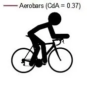
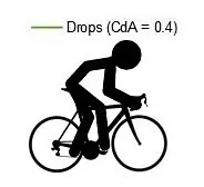
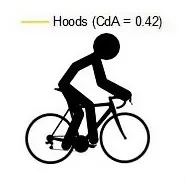
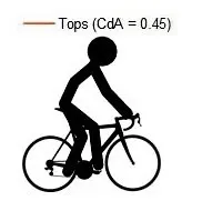
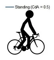
When the cyclist holds the first position (i.e Aerobars position) on the cycle the area exposed to the free air is minimum and hence the Drag coefficient and drag force are minimum. Similarly, as the cyclist changes his position the area is changes and more areas is get exposed in the opposite direction to the airflow. This causes an increase in drag coefficient and drag force as shown in the below Plots.
Note:- The area of a cyclist is only changing due to change of his position while the cycle area is constant in all the cases.
i. Matlab Output:-
ii. Python Output:-
a. Plot For Velocity (Vs) Drag force:
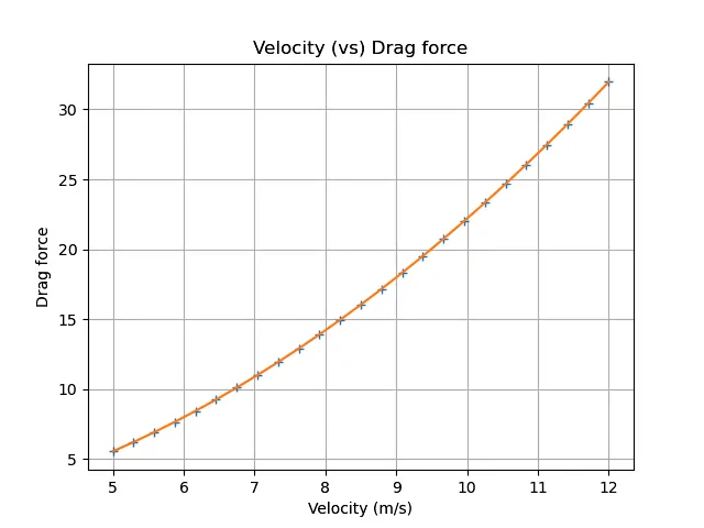
In the case of Velocity, as the velocity of the cycle increases keeping area constant, the impact of the airflow is getting higher and the backward force (i.e Drag force) acting on the cyclist is increases by making curvature as shown above.
b. Plot For Drag Coefficient (vs) Drag force:
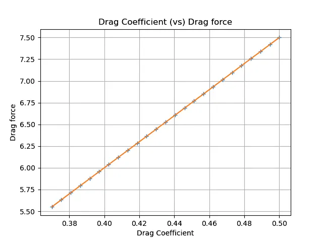
Here, from the above figure, we can see that as the frontal area changes the drag coefficient is changed. Also, the variation of the Drag force is linear with respect to the drag coefficient. This indicates that the Drag Coefficient is directly proportional to the Drag Force.
Hence, From the above Results, to reduce the effort and increase the velocity of a cycle we need to decrease the area exposed to the free air while cycling which causes the lower Drag coefficient and Drag force.
References:-
https://ridefar.info/bike/cycling-speed/air-resistance-cyclist/
The fLow of Report:-
1. Objective.
2. Basic.
3. Considered Parameters.
4. Program And Explanation.
5. Error & Error Elimination.
6. Result & Conclusion.