BREAKING ICE WITH AIR CUSHION VEHICLE - FIND MINIMUM PRESSURE WITH NEWTON-RAPHSON METHOD.

1. Objective:-

Writing a python script to solve for the minimum value of pressure needed to break a given thickness of ice using the newton raphson method.

`p3(1 − β^2)+(0.4*h*β^2 − (σ*h^2)/r^2 )*p^2 + (σ^2* h^4)/(3r^4)*p − ((σ *h^2)/(3r^2))^3 = 0`

Take β = 0.5, r = 40 feet and σ = 150 pounds per square inch (psi).

We need to,

1. Use the newton raphson method to find out the value of pressure for h = 0.6 ft.

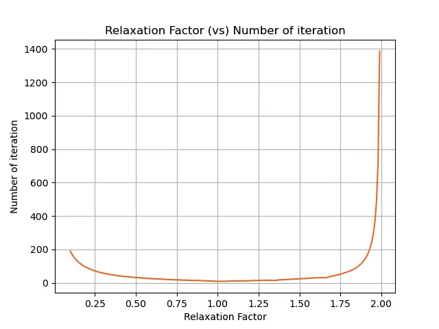
2. Find the optimal relaxation factor for this problem with the help of a suitable plot.

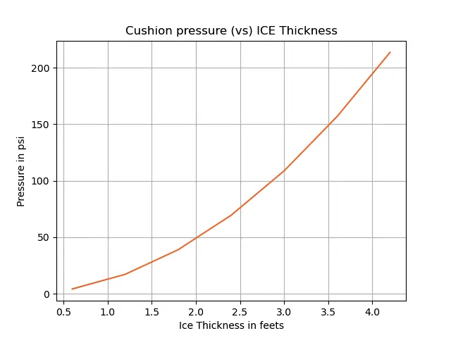
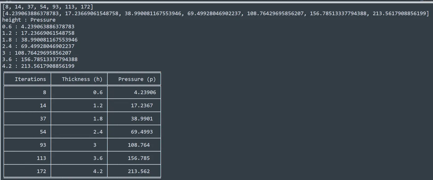
3. Tabulate the results of p for h = [0.6,1.2,1.8,2.4,3,3.6,4.2] assuming a suitable relaxation factor.

2. Basics:-

2.1 Air-Cushion Vehicle:-

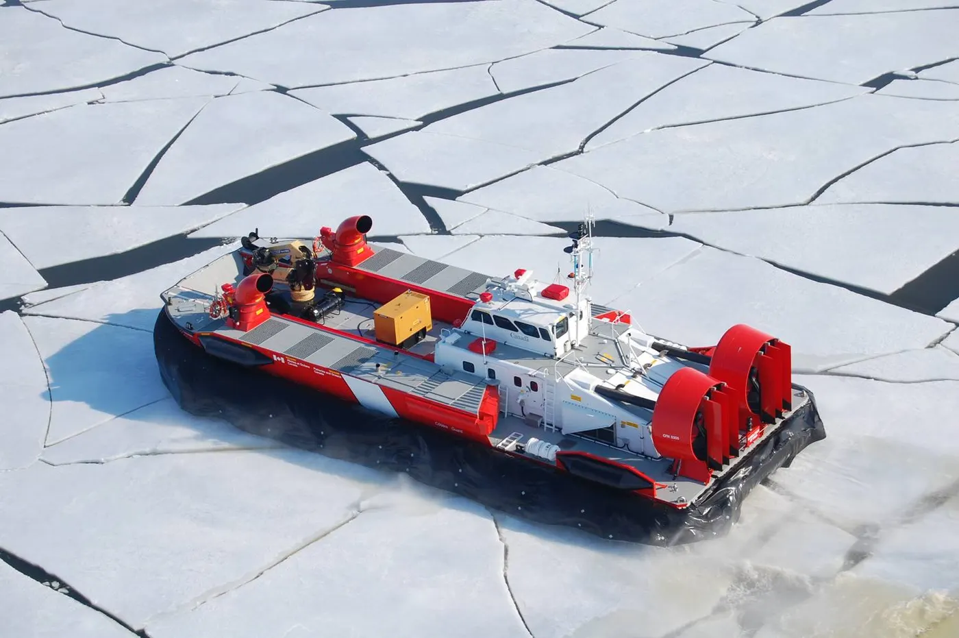
A hovercraft, also known as an air-cushion vehicle or ACV, is a craft capable of running on almost every surface such as ground, water surface, mud, sands, grits, weeds etc. Hovercraft use blowers to produce a large volume of air below the hull that is slightly above atmospheric pressure. The pressure difference between the higher pressure air below the hull and lower pressure ambient air above it produces lift, which causes the hull to float above the running surface. For stability reasons, the air is typically blown through slots or holes around the outside of a disk or oval-shaped platform, giving most hovercraft a characteristic rounded-rectangle shape. Typically this cushion is contained within a flexible "pocket", which allows the vehicle to travel over small obstructions without damage.

To determine the minimum cushion pressure needed to break a given thickness of ice using an air cushion vehicle we are using the following formula and use it in the program with the help of Newton–Raphson method.

`p3(1 − β^2)+(0.4β^2 − σ*h^2/r^2 )p^2 + σ^2* h^4/(3r^4)*p − (σ *h^2/(3r^2))^3 = 0`

Where:-

p = cushion pressure in psi

β = width of the ice-wedge

σ = tensile strength of the ice

r = size of the air cushion

h = is the thickness of the ice field

2.2 Newton–Raphson method:-

In numerical analysis, Newton's method, also known as the Newton–Raphson method, named after Isaac Newton and Joseph Raphson, is a root-finding algorithm which produces successively better approximations to the roots (or zeroes) of a real-valued function. The most basic version starts with a single-variable function f defined for a real variable x, the function's derivative f ′, and an initial guess x0 for a root of (f). If the function satisfies sufficient assumptions and the initial guess is close, then

is a better approximation of the root than x0. Geometrically, (x1, 0) is the intersection of the x-axis and the tangent of the graph of f at (x0, f (x0)): that is, the improved guess is the unique root of the linear approximation at the initial point. The process is repeated as

until a sufficiently precise value is reached. This algorithm is first in the class of Householder's methods, succeeded by Halley's method. The method can also be extended to complex functions and to systems of equations.

The idea is to start with an initial guess which is reasonably close to the true root, then to approximate the function by its tangent line using calculus, and finally
to compute the x-intercept of this tangent line by elementary algebra. This x-intercept will typically be a better approximation to the original function's root than
the first guess, and the method can be iterated.

More formally, suppose f : (a, b) → ℝ is a differentiable function defined on the interval (a, b) with values in the real numbers ℝ, and we have some current approximation x_n. Then we can derive the formula for a better approximation, x_{n + 1} by referring to the diagram on the right. The equation of the tangent line to the curve y = f (x) at x = x_n is

where f′ denotes the derivative. The x-intercept of this line (the value of x which makes y = 0) is taken as the next approximation, x_{n + 1}, to the root so that the equation of the tangent line is satisfied when :

Solving for x_{n + 1} gives

We start the process with some arbitrary initial value x₀. (The closer to the zero, the better. But, in the absence of any intuition about where the zero might lie, a "guess and check" method might narrow the possibilities to a reasonably small interval by appealing to the intermediate value theorem.) The method will usually converge, provided this initial guess is close enough to the unknown zero, and that f ′(x₀) ≠ 0. Furthermore, for a zero of multiplicity 1, the convergence is at least quadratic (see a rate of convergence) in a neighbourhood of the zero, which intuitively means that the number of correct digits roughly doubles in every step. More details can be found in the analysis section below.

In our Formula, we are using the alpha which is known as relaxation factor. hence our revised formula is as follows.

`x_(n+1) = x_n - alpha*(f(x_n))/(f'(x_n))`

3. Procedure and Explanation:-

3.1 First Program:

Step-1: Initialization of the first program.

Importing the required libraries

import math
import matplotlib.pyplot as plt
from tabulate import tabulate
import numpy as numpy

Where:-
i. The "import math" and "import matplotlib.pyplot as plt" are used to use the mathematical constants and plotting the graph respectively.

ii. If you want to create some tables from a python list, you can use the tabulate module, it can generate the table easily in text mode and in many formats. The module provides just one function, "tabulate" which takes a list of lists or another tabular data type as the first argument, and outputs a nicely formatted plain-text table:

iii. "import numpy as np" is used to give power to each element of an array or to perform any mathematical operations (like addition or subtraction) either on every element of an array or between the arrays.

Step-2: Defining Functions.

Before defining the function we need to simplify the Equation used in it. Hence, to simplify the formula we divided formula into five sub formulas (terms) and combined it to get a proper formula.

`p3(1 − β^2)+(0.4*h*β^2 − (σ*h^2)/r^2 )*p^2 + (σ^2* h^4)/(3r^4)*p − ((σ *h^2)/(3r^2))^3 = 0`

Let

term1 = `p3(1 − β^2)`

term2 = `(0.4*h*β^2 ) *p^2`

term3 = `(σ*h^2)/r^2 )*p^2`

term4 = `((σ^2* h^4)/(3r^4))*p`

term5 = `((σ *h^2)/(3r^2))^3`

After optimizing the formula we are defining the function as shown below.

Note:- in Program we denoted the (σ) as an (s).

1. f(x) (i.e Equation 1):

def f(p,b,r,s,h):
	term1=pow(p,3)*(1-pow(b,2))
	term2=0.4*h*pow(b,2)*pow(p,2)
	term3=s*pow(p,2)*pow(h,2)/pow(r,2)
	term4=(p*pow(s,2)*pow(h,4))/(3*pow(r,4))
	term5=(s*pow(h,2))/(3*pow(r,2))
	term5=pow(term5,3)
	eq1=term1+term2-term3+term4-term5
	return eq1

2. f'(x) (i.e Equation 2): We need to define the derivative of the formula to use in the Newton Rapson method which is as follows.

def fprime(p,b,r,s,h):
	term6=3*pow(p,2)*(1-pow(b,2))
	term7=0.8*p*h*pow(b,2)
	term8=2*s*p*pow(h,2)/pow(r,2)
	term9=(pow(s,2)*pow(h,4))/(3*pow(r,4))
	eq2=(term6+term7-term8+term9)
	return eq2

Where:-

i. f is the primary equation which is defined in the function similarly, fprime is the Secondary equation (a derivative of the primary equation) which is defined in the function.

ii. "return" command is used to return the calculated function value and save it. Used to get multiple values.

Step-3: Defining Inputs.

b = 0.5 		
r = 40 		
s = 21600 	
h = [0.6,1.2,1.8,2.4,3,3.6,4.2] 
p_guess = 10
alpha = 1 

Where:-
b = width of ice-wedge.

r = size of air cushion.

s = Tensile strength In PSF.

Because the tensile strength is in PSI we need to convert it into PSF to maintain dimensional stability. hence PSF = PSI*144 (i.e 21600 PSF = 150*144 PSI)

h = thickness of the ice.

p_gess = Initial value considered for first iteration.

alpha = relaxation factor

Step-4: Defining loops.

p = []
iterations = []

for i in h:
	while(abs(f(p_guess,b,r,s,i))>tol):
		p_guess=p_guess-alpha*(f(p_guess,b,r,s,i)/fprime(p_guess,b,r,s,i))
		itr=itr+1
	iterations.append(itr)
	p.append(p_guess)

print(iterations)
print(p)

for i in range(0,7):
	if i==0:
		print("height : Pressure")
	print(h[i],":",p[i])

Where:-

i. tol = 1e-6 is a Tolerance. Since it is iterative process f(x) is not going to be zero it is near about zero. There are always error associated with it which is defined as Tolerance.
i.e if f(x) evaluate 1e-6 then (i) will take this answer.

ii. We are using while-loop to define the condition "(abs(f(p_guess,b,r,s,i))>tol)".

iii. "iter" acts as a loop counter.

iv. "p = [] , iterations = []" is Defines the empty array to dump the calculated value from the loop.

v. To generate the multiple values we need one more command called append.".append" is used to continuously append (increase) the value and store it in the empty array.

vi. similarly, we defined another for-loop and print command used to print the multiple values.

Step-5: Table Plotting.

# Plotting Table
headers=['Iterations','Thickness (h)','Pressure (p)']
table=tuple(zip(iterations,h,p))
print(tabulate(table,headers=headers,tablefmt="fancy_grid"))

Where:-

To plot the table we need some new command which is discussed below.

i. Python List is a data structure that maintains an ordered collection of mutable data elements. Python Tuple is an immutable data structure whose elements are enclosed within parenthesis ().
We can create a list of tuples i.e. the elements of the tuple can be enclosed in a list and thus will follow the characteristics in a similar manner as of a Python list. Since, Python Tuples utilize less amount of space, creating a list of tuples would be more useful in every aspect.

ii. Python zip() function can be used to map the lists altogether to create a list of tuples using the below command: list(zip(list))

iii. The zip() function returns an iterable of tuples based upon the values passed to it. And, further, the list() function would create a list of those tuples as an output from the zip() function.

Example:
input:
lst1 = [10,20,30]
lst2 = [50,"first value","second value"]
lst_tuple = list(zip(lst1,lst2))
print(lst_tuple)

Output:[(10, 50), (20, 'first value'), (30, 'second value')]

iv. The "tabulate" takes a list of lists or another tabular data type as the first argument, and outputs a nicely formatted plain-text table.

v. "headers" defines a list of column headers to be used.

vi. "fancy_grid" draws a grid using box-drawing characters. i.e it is a type of table formate.

Step-6: Plotting.

# Plotting
plt.grid()
plt.plot(h,p,color=[0.9100,0.4100,0.1700])
plt.title("Cushion pressure (vs) ICE Thickness")
plt.xlabel("Ice Thickness in feets")
plt.ylabel("Pressure in psi")
plt.savefig("Case-1")
plt.show()

Using the plot command to plot the graph of Cushion pressure (vs) ICE Thickness.

Where:-

i. plt.grid() used to show the grid in the plot.

ii. plt.plot() used as plot command.

iii. plt.title defines the title for the plot.

iv. Defining the label for the x and y-axis using "plt.xlabel()" and "plt.ylabel()" commands.

v. plt.savefig() command used to save the plot in the computer.

vi. plt.show() used to show the plot.

3.2 Second Program:

In this program, we need to find out the optimum value of the relaxation factor. All the terms discussed in the first program is applicable to this program also. Hence we are explaining only those terms which is getting change in our second program.

Step 1: Defining loop.

In this program, we need to find out the optimum value of the relaxation factor. to do that we are defining loop for the alpha which contains newton rapshon formula. the loop explanation is already done in the primary program.

#Defining Loop
for i in alpha:
	p_guess=10
	itr=1
	while((abs(f(p_guess,b,r,s,h)))>tol):
		p_guess=p_guess-i*(f(p_guess,b,r,s,h)/fprime(p_guess,b,r,s,h))
		itr=itr+1
	iterations.append(itr)
	p.append(p_guess)
	a.append(i)

Where:-

i. we are considering the thickness of ice minimum as h=0.6

Step 2: Defining the optimum Relaxation factor.

#Optimum relaxation factor
print(iterations)
print(p_guess)
print("The minimum iterations is:",min(iterations))

index_min_iteration=iterations.index(min(iterations))
alpha_optimum=alpha[index_min_iteration]

print("Optimum alpha=",alpha_optimum)

Where:-

i. The min() function returns the item with the lowest value or the item with the lowest value in an iterable. An iterable, with one or more items to compare. If the values are strings, an alphabetical comparison is done.

Step 3: Plotting.

plt.grid()
plt.plot(a,iterations,color=[0.9100,0.4100,0.1700])
plt.title('Optimum Relaxation Factor')
plt.xlabel("Relaxation Factor")
plt.ylabel("Number of iteration")
plt.savefig("Case-2")
plt.show()

The plotting command used is based on the command discussed in step-6 of the primary program.

4. Final Program and Output:-

4.1 Program-1:

i. program:

# Program 1
# Importing Libraries.

import math
import matplotlib.pyplot as plt
from tabulate import tabulate
import numpy as numpy

# Defining function for first Equation
def f(p,b,r,s,h):								# f is fuction contains main formula
	term1=pow(p,3)*(1-pow(b,2))					
	term2=0.4*h*pow(b,2)*pow(p,2)
	term3=s*pow(p,2)*pow(h,2)/pow(r,2)
	term4=(p*pow(s,2)*pow(h,4))/(3*pow(r,4))
	term5=(s*pow(h,2))/(3*pow(r,2))
	term5=pow(term5,3)
	eq1=term1+term2-term3+term4-term5			# Final Equation 1
	return eq1									# Returning the Value of Equation 1


# Defining function for Second Equation			# fprime function contains derivative of the main formula.
def fprime(p,b,r,s,h):
	term6=3*pow(p,2)*(1-pow(b,2))
	term7=0.8*p*h*pow(b,2)
	term8=2*s*p*pow(h,2)/pow(r,2)
	term9=(pow(s,2)*pow(h,4))/(3*pow(r,4))
	eq2=(term6+term7-term8+term9)				# Final Equation 2
	return eq2									# Returning the Value of Equation 2

"""
Using Newton Raphson iteration
Where:-
b = width of ice wedge
r = size of air cushion
s = Tensile strength In PSF = PSI*144
h = thickness of ice
alpha = relaxation factor

"""

b = 0.5 		
r = 40		
s = 21600 	
h = [0.6,1.2,1.8,2.4,3,3.6,4.2] 
p_guess = 10
tol = 1e-6
alpha = 1 
itr = 1
p = []
iterations = []

for i in h:
	while(abs(f(p_guess,b,r,s,i))>tol):
		p_guess=p_guess-alpha*(f(p_guess,b,r,s,i)/fprime(p_guess,b,r,s,i))
		itr=itr+1
	iterations.append(itr)
	p.append(p_guess)

print(iterations)
print(p)

for i in range(0,7):
	if i==0:
		print("height : Pressure")
	print(h[i],":",p[i])


# Plotting Table
headers=['Iterations','Thickness (h)','Pressure (p)']			# Defining Headers
table=tuple(zip(iterations,h,p))
print(tabulate(table,headers=headers,tablefmt="fancy_grid"))	# Plotting table using fancy_grid

# Plotting
plt.grid()
plt.plot(h,p,color=[0.9100,0.4100,0.1700])
plt.title("Cushion pressure (vs) ICE Thickness")
plt.xlabel("Ice Thickness in feets")
plt.ylabel("Pressure in psi")
plt.savefig("Case-1")
plt.show()

ii. Output:

4.2 Program-2:

i. program:

import math
import matplotlib.pyplot as plt
import numpy as np

def f(p,b,r,s,h):								# f is fuction contains main formula
	term1=pow(p,3)*(1-pow(b,2))
	term2=0.4*h*pow(b,2)*pow(p,2)
	term3=s*pow(p,2)*pow(h,2)/pow(r,2)
	term4=(p*pow(s,2)*pow(h,4))/(3*pow(r,4))	
	term5=(s*pow(h,2))/(3*pow(r,2))
	term5=pow(term5,3)
	eq1=term1+term2-term3+term4-term5			# Final Equation 1
	return eq1									# Returning the Value of Equation 1


def fprime(p,b,r,s,h):							# fprime function contains derivative of the main formula.
	term6=3*pow(p,2)*(1-pow(b,2))
	term7=0.8*p*h*pow(b,2)
	term8=2*s*p*pow(h,2)/pow(r,2)
	term9=(pow(s,2)*pow(h,4))/(3*pow(r,4))
	eq2=(term6+term7-term8+term9)				# Final Equation 2
	return eq2									# Returning the Value of Equation 2

"""
Using Newton Raphson iteration
Where:-
b = width of ice wedge
r = size of air cushion
s = Tensile strength In PSF = PSI*144
h = thickness of ice
alpha = relaxation factor

"""

b=0.5 		
r=40 		
s=21600 	
h=0.6 		

tol=1e-6
alpha=np.linspace(0.1,1.99,200) #relaxation factor

p=[]
a=[]
iterations=[]

#Defining Loop
for i in alpha:
	p_guess=10
	itr=1
	while((abs(f(p_guess,b,r,s,h)))>tol):
		p_guess=p_guess-i*(f(p_guess,b,r,s,h)/fprime(p_guess,b,r,s,h))
		itr=itr+1
	iterations.append(itr)
	p.append(p_guess)
	a.append(i)

#Optimum relaxation factor
print(iterations)
print(p_guess)
print("The minimum iterations is:",min(iterations))

index_min_iteration=iterations.index(min(iterations))
alpha_optimum=alpha[index_min_iteration]

print("Optimum Relaxation Factor=",alpha_optimum)

plt.grid()
plt.plot(a,iterations,color=[0.9100,0.4100,0.1700])
plt.title('Relaxation Factor (vs) Number of iteration')
plt.xlabel("Relaxation Factor")
plt.ylabel("Number of iteration")
plt.savefig("Case-2")
plt.show()

ii. Output:

5. Result and conclusion:-

From the Program and its Output, we can Conclude the following Results.

1. As the thickness increases the pressure required to break the given thickness of ice increases and makes slightly curvature path. This indicates that the direct relationship between the pressure and thickness of the ice.

2. From the plot, we can say that as the relaxation factor value (Alpha) increases, The number of Iteration is decreased to obtain the required value i.e We will jump to the Required value earlier. This may provide considerable result but in the complex curve higher value of relaxation, factor conclude bad result. Hence to get the best possible value of the relaxation factor we need to study optimization.

3. Based on the optimization result we can conclude that the optimum relaxation factor in our case found is 0.9927638190954773.

4. The Optimum relaxation factor Value found during the program is less that one (i.e `alpha <1`), which is the best choice for us and also known as under relaxation factor.

Reference:-

https://en.wikipedia.org/wiki/Newton%27s_method

https://www.askpython.com/python/list/python-list-of-tuples

https://github.com/astanin/python-tabulate

https://www.w3schools.com/python/ref_func_min.asp

The Flow of Report:-

1. Objective.

2. Basics.

3. Procedure and Explanation.

4. Final Program and Output.

5. Result and conclusion.