Week 8 - Simulating Cyclone separator with Discrete Phase Modelling
Aim :
To perform analysis on cyclone separator and calculate the separation efficiency and pressure drop.
Objective :
- To write a few words about any four empirical models used to calculate the cyclone separator efficiency.
- To perform an analysis on a given cyclone separator model by varying the particle diameter from 1 μm to 5 μm and calculate the separation efficiency in each case. Discuss the results. [Use both the velocity's as 3m/sec.]
- To perform an analysis on a given cyclone separator model by varying the particle velocity from 1 m/sec to 5 m/sec and calculate the separation efficiency and pressure drop in each case. Discuss the results. [Use particle diameter size as 5 μm for all cases & keep flow velocity same as particle velocity]
Cyclone seperator :
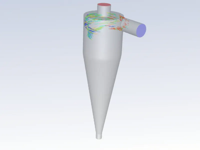
- Cyclone is a common separation and classification equipment, and the principle of centrifugal sedimentation is often used.
- When the two-phase mixture to be separated enters the hydrocyclone tangentially from the periphery of the hydrocyclone at a certain pressure, a strong three-dimensional elliptical strong rotational shear turbulent motion is produced.
- Because of the particle size difference between coarse particles and fine particles, they are affected by centrifugal force, centripetal buoyancy force, fluid drag force and so on. Under the action of centrifugal sedimentation, most of the coarse particles are discharged through the bottom outlet of the hydrocyclone, while most of the fine particles are discharged from the overflow pipe, so as to achieve the purpose of separation and classification.
- The efficiency of cyclone seperator depends on inlet velocity, density of the particulate matter and geometrical dimension of the set-up.
Applications :
1. Classification and sorting :
When classifying, it is used in conjunction with grinding equipment to carry out pre-classification or classification of coarse and fine particles in ball mills. When sorting the material, the material is fed into the cylinder at a certain pressure along the tangent direction, and the material moves along the inner wall of the cylinder. Under the joint action of centrifugal force and gravity, the material with higher density moves downward spirally along the inner wall of the cylinder. Finally, it is discharged from the ore discharge port at the bottom, and the less dense material moves upward along the central part through the separation interface. Finally, the finer ore particles discharged by the overflow pipe form a spiral upward slurry flow in the center of the cone and water, which is discharged through the overflow pipe.
2. Desliming :
Hydrocyclones can remove mud and flotation reagents from various minerals, and concentrate can be recovered and coarse sand can be removed from non-metallic minerals.
3. Concentration :
The hydrocyclone can concentrate the pulp with too low concentration in order to meet the process requirements.
4. Sand removal and impurity removal :
In the mineral processing process, there may be some magazines in minerals, in order to meet the design requirements, impurities must be dealt with, then the hydrocyclone can play a good role. With different ore properties, different cyclones are used.
5. Tailings filling and dam construction :
The materials for tailings dam construction have particle size requirements. Hydrocyclones are used for classification to screen out particles that do not meet the particle size requirements.
Four empirical models used to calculate the cyclone separator efficiency :
IOZIA AND LEITH MODEL :
- Iozia and Leith (1990) logistic model which is developed based on force balance.
- The model assumes that a particle carried by the vortex endures with the influence of two forces which is a centrifugal force and a flow resistance.
`η_i = 1/(1+(d_(pc) / d_(pi))^(beta))`
LI AND WANG MODEL :
- The Li and Wang (1989) model includes particle bounce or re-entrainment and turbulent diffusion at the cyclone wall.
- A two-dimensional analytical expression of particle distribution in the cyclone is obtained.
- The resultant expression of the collection efficiency for particle of my size is given as
`η_i = 1 - exp {-λθ_1}`
KOCH AND LICHT MODEL :
Koch and Licht (1977) collection theory recognized the inherently turbulent nature of cyclones and the distribution of gas residence times within the cyclone. Koch and Licht describe particle motion in the entry and collection regions with the additional following assumptions:
- The tangential velocity of a particle is equal to the tangential velocity of the gas flow, i.e. there is no slip in the tangential direction between the particle and the gas.
- The tangential velocity is related to the radius of cyclone by : u`R^n` = constant.
- A force balance and an equation on the particles collection yields the grade efficiency(`η_i`) is given by
`η_i` = `1-exp{-2[(GT_iQ)/D^3(n+1)]^(0.5/(n+1))}`
LAPPLE MODEL :
- Lapple (1951) model was developed based on force balance without considering the flow resistance.
- Lapple assumed that a particle entering the cyclone is evenly distributed across the inlet opening.
- The efficiency of collection of any size of particle is given by
`η_i = 1/(1+(d_(pc) / d_(pi))^(2))`
Project Methodology :
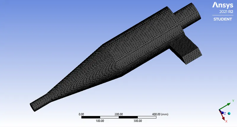
The project is intended to study the effect of particulate diameter size and gas flow velocity (discrete and continuous phase) on the efficacy of the cyclone separator. Numerical analysis is carried in ANSYS FLUENT with post-processing in CFD-post. Initially the geometry clean up is performed to reduce the inclusion of extra (unwanted) features into the meshing and solving platform. The cleaned geometry is imported in ANSYS Meshing and cartesian mesh is used to mesh the geometry. As cartesian mesh is aligned to the flow direction which certainly leads to more accurate results and better convergence in CFD solvers. The resulted mesh is finally imported in FLUENT module where numerical analysis is performed using Discrete Phase Model (DPM). The obtained results are post-processed and are discussed accordingly.
Case studies :
Case Study One: Varying particle diameter with same inlet velocity.
| Cases | Particle diameter (microns) | Particle (Discrete) and continuous fluid velocity (m/sec) |
| Case 1a | 1 | 3 |
| Case 1b | 3 | 3 |
| Case 1c | 5 | 3 |
Case Study Two: Varying inlet velocity with same particle diameter.
| Cases | Particle diameter (microns) | Particle (Discrete) and continuous fluid velocity (m/sec) |
| Case 2a | 5 | 2 |
| Case 2b | 5 | 4 |
| Case 2c | 5 | 5 |
Pre-processing :
Geometry :
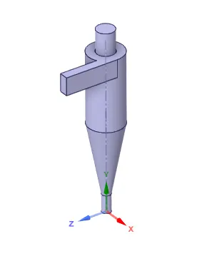
- Import the geometry in the space claim and extract the fluid volume by using volume extract.
- Then suppress the solid body which helps to increases the computational time by avoid meshing in the solid region.
Mesh :
Mesh Details :
| Global element size | 5 mm |
| Maximum element size | 5 mm |
| Cartesian method | As per global settings |
| Face sizing | As per local settings |
| Local face mesh element size | 3.5 mm |
| Total number of nodes | 504117 |
| Total number of elements | 473504 |
Note: Same mesh is used for all case studies to expect consistent and mesh independent results. The mesh settings are selected under different trials to achieve accurate results.
Sectional view :
Named selections :
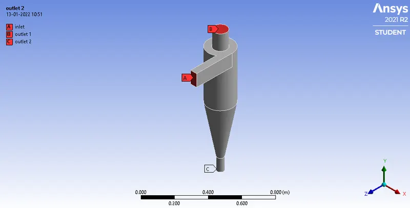
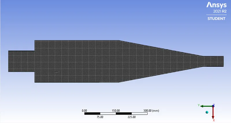
The patches colored in red represents the faces which are subjected to subsequent boundary conditions in FLUENT solver. It helps to identify cell face zones and assignment of respective boundary conditions to it.
Mesh quality :
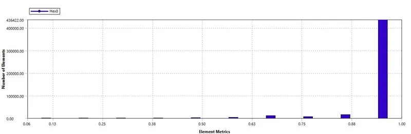
Element quality :
Setup :
SETUP | |
Gravity | -9.81 in the Y direction |
Solver Type | Pressure-Based |
Velocity Formulation | Absolute |
Time | Steady |
Models | Viscous model: K-epsilon, RNG, Swirl Dominated flow. Energy model: OFF Discrete Phase model: on |
Pressure-velocity coupling | Simple Turblence kinetic energy - second order upwind. Turblence dissipation rate - second order upwind |
Material | Fluid type: Air Solid-type: Aluminium |
Cell zones | Fluid type: Air Solid: Al |
Boundaries | Inlet velocity : Varies according to the case DPM: reflect Wall:- DPM: Reflect Outlet(Top): DPM: Escape Outlet(Bottom/dustbin) -DPM: Trap |
Reference values | Standard |
Initialization | Standard Starting from inlet |
Note :
In Discrete Phase Model ⇒ Tick the check boxes Iteraction with continuous phase, update DPM sources every flow iteration ⇒ Max no. of steps ⇒ Run up to 50000 iterations.
Create Injections ⇒ surfaces(Injection type) ⇒ Inlet(Release from surfaces)
The particle material is choosen as Anthracite ⇒ particle type is selected as inert ⇒ provide velocity magnitude which is our particle velocity and particle diameter both varies depends upon the case.
Case 1 :
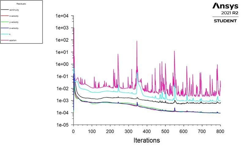
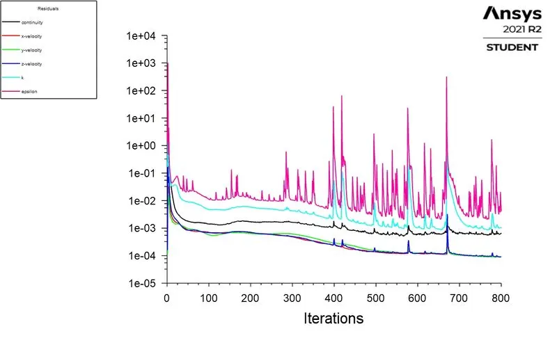
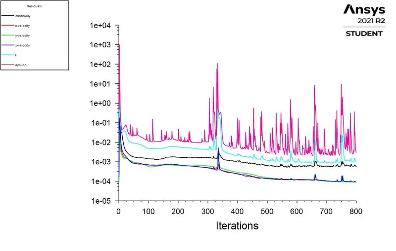
1. Scaled residuals :
For case(1a) :
For case(1b) :
For case(1c) :
2. DPM Report :
For case(1a)

For case(1b)

For case(1c)

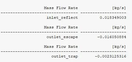
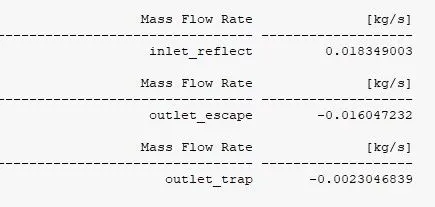
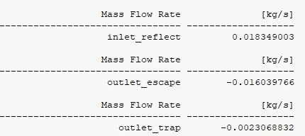
3. Mass Flow Rate Report :
For case(1a)
For case(1b)
For case(1c)
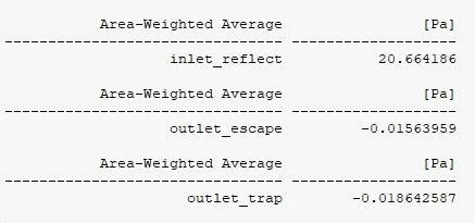
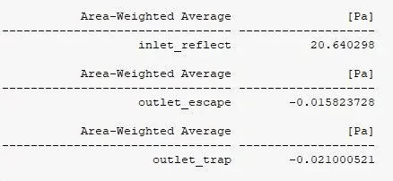
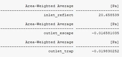
4. Area average pressure report :
For case(1a)
For case(1b)
For case(1c)
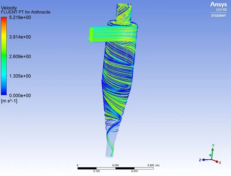
5. Velocity Contour :
For case(1a)
For case(1b)
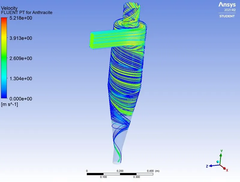
For case(1c)
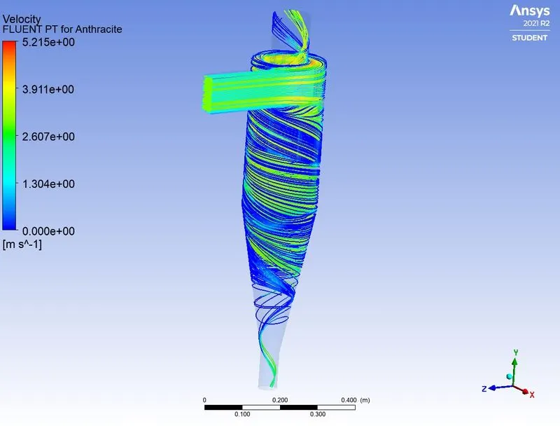
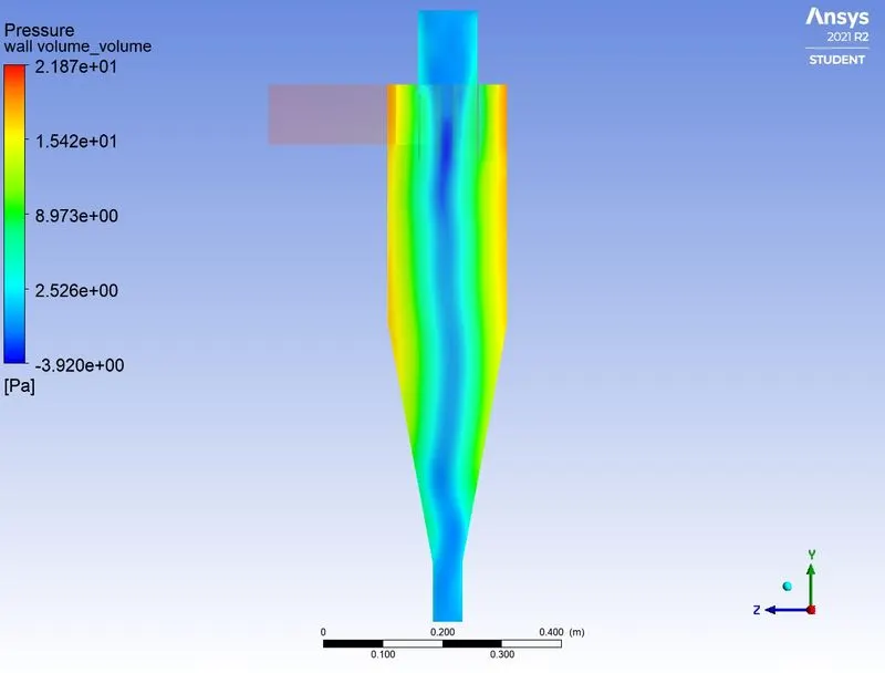
6. Pressure Contour Plane :
For case(1a)
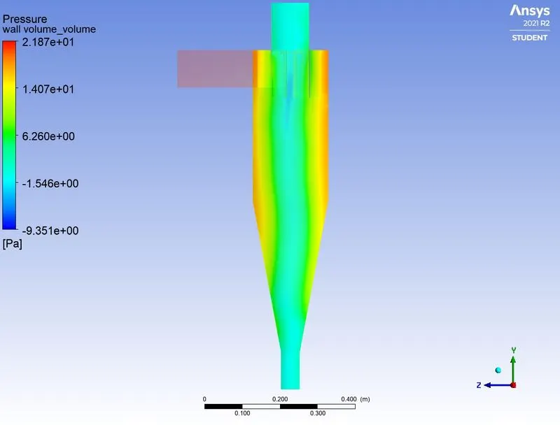
For case(1b)
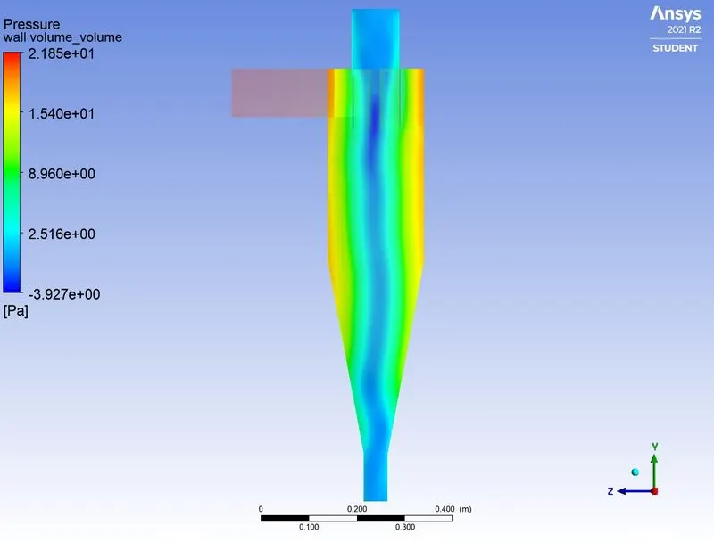
For case(1c)
6. Particle Residence Time :
For case(1a)
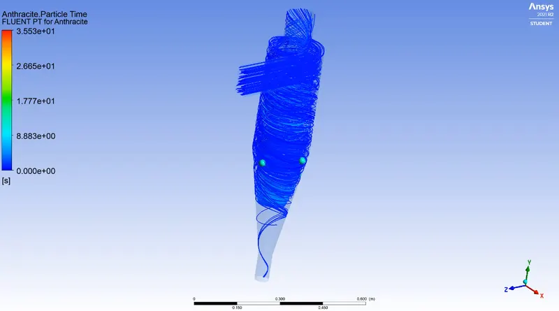
Animation : https://youtu.be/lnCAoyr6F8I
For case(1b)
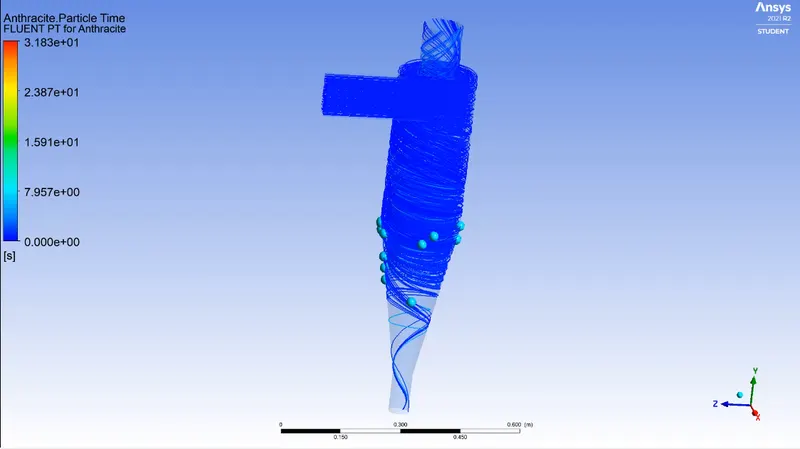
Animation : https://youtu.be/92A0ZFJtR7A
For case(1c)
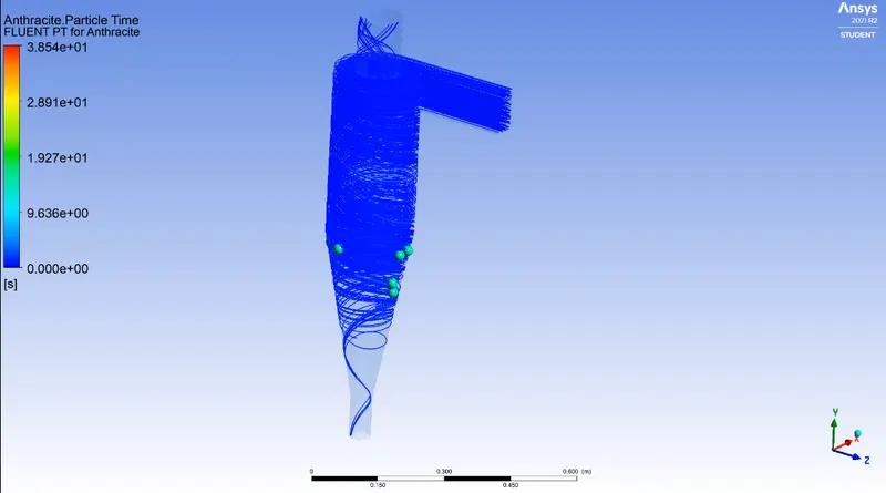
Animation : https://youtu.be/SYBNOgqrEd4
Observation table :
| Cases | Particle Diameter (microns) | Particle Velocity (m/s) | Particles Escaped | Particles Trapped | Incomplete Particles | Efficiency (η in %) |
| Case 1a | 1 | 3 | 185 | 40 | 167 | 10.204 |
| Case 1b | 3 | 3 | 128 | 55 | 209 | 14.03 |
| Case 1c | 5 | 3 | 64 | 63 | 265 | 16.07 |
The separation effciency is given as,
η = Trapped particles / Total number of particles
Note: The above calculated efficiency is calculated by neglecting the number of incomplete particles.
Case 2 :
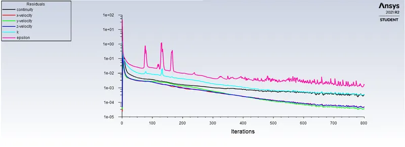
1. Scaled residuals :
For case(2a)
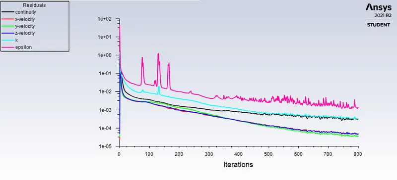
For case(2b)
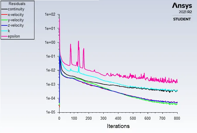
For case(2c)
2. DPM Report :
For case(2a)

For case(2b)

For case(2c)

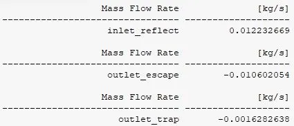
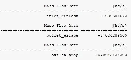
3. Mass Flow Rate Report :
For case(2a)
For case(2b)
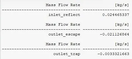
For case(2c)
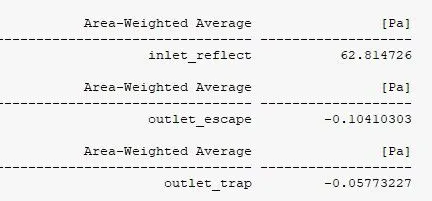
4. Area average pressure report :
For case(2a)
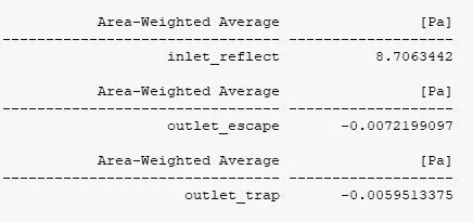
For case(2b)
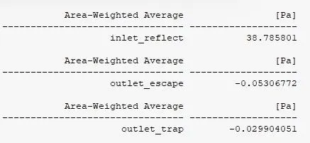
For case(2c)
5. Velocity Contour :
For case(2a)
For case(2b)
For case(2c)
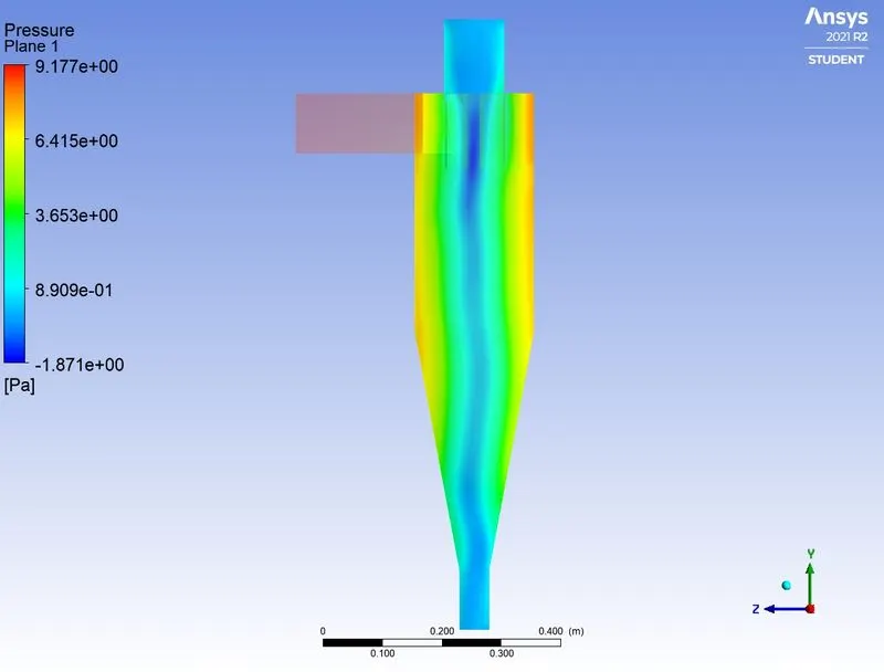
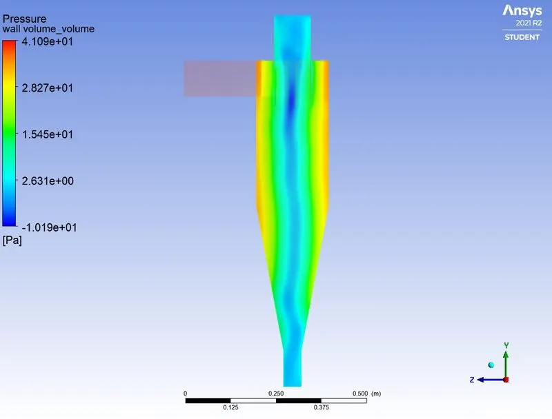
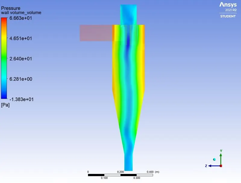
6. Pressure Contour Plane :
For case(2a)
For case(2b)
For case(2c)
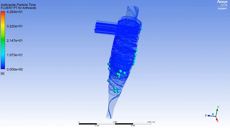
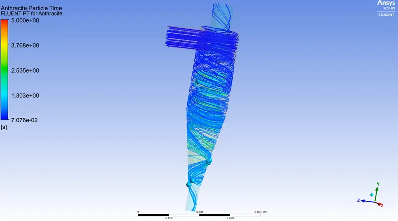
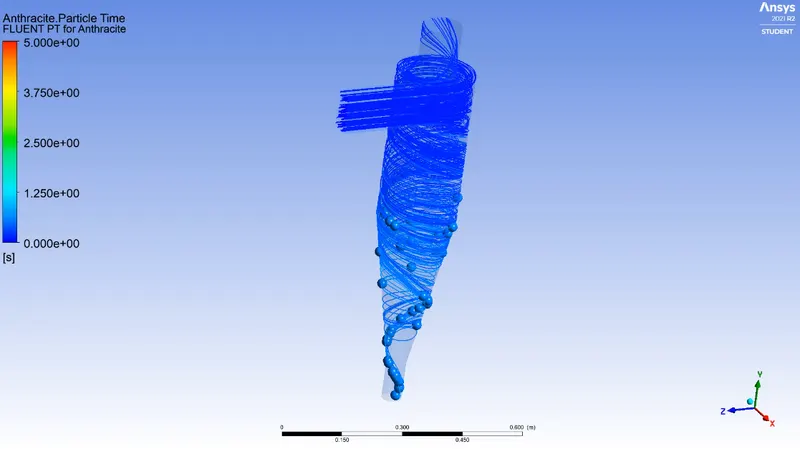
7. Particle Residence Time :
For case(2a)
Animation : https://youtu.be/uyjK9TTeDrk
For case(2b)
Animation : https://youtu.be/wTxh216N6vo
For case(2c)
Animation : https://youtu.be/Ox0kYAGvXgs
Observation table :
| Cases | Particle Diameter (microns) | Particle Velocity (m/s) | Particles Escaped | Particles Trapped | Incomplete Particles | Efficiency (η in %) |
| Case 1a | 1 | 3 | 82 | 46 | 264 | 11.735 |
| Case 1b | 3 | 3 | 62 | 287 | 43 | 73.21 |
| Case 1c | 5 | 3 | 60 | 331 | 1 | 84.44 |
The separation effciency is given as,
η = Trapped particles / Total number of particles
Note: The above calculated efficiency is calculated by neglecting the number of incomplete particles.
Conclusion :
The Euler-Lagrangian model has been used to simulate the case of cyclone separator with K-epsilon (RNG) turbulence model. The separation efficiency and pressure drop has been calculated for various cases with vaying particle diameter and inlet velocity. The obtained results are promising and are able to imitate appropriate physics. The following conclusions can be drawn from the present study:
Case Study 1: Varying particle diameter with same inlet velocity (3ms).
1. The smaller particles tend to escape due to less density and inertia which results in lower separation efficiency. In contrast to it, larger particles possess higher density and inertial effects due to which they get collected to the bottom under the gravitational influence.
2. The particle residence time is more in case of larger particles.
3. There is no much variation in pressure drop.
Case Study 2 : Varying inlet velocity with particle diameter being 5 μm.
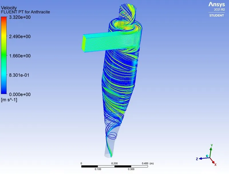
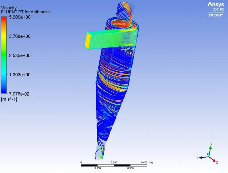
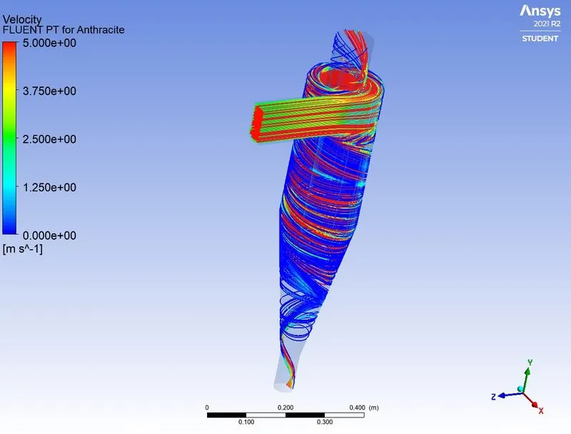
1. The particles with lesser velocity escapes or get stucked in the re-circulation region due to less pressure difference and leads to less separation efficiency. However the particles with high velocity are accelerated to the outlet due to high pressure difference and get trapped at the bottom. This certainly increases the separation efficiency for the particles with high velocity.
2. The particle residence time is more in case of particles with lesser velocity after the particular velocity is attained with increased efficiency its velocity is more or less equal.
3. Pressure drop increases with the increase in the fluid inlet velocity and also higher pressure drop will increase the seperation efficiency.
References :