Week 4 - CHT Analysis on Exhaust port
- To give a brief description of why and where a CHT analysis is used.
- To maintain the y+ value according to the turbulence model and justify the results.
- To calculate the wall/surface heat transfer coefficient on the internal solid surface & show the velocity & temperature contours in appropriate areas.
- To verify the calculated results with a analytical/Experimental value.
Conjugate Heat Transfer (CHT) :
- Thermal interaction between the fluid and the solid region it can be either natural convection or forced convection.
- In solid region we are simulating the heat conduction. The heat conduction is basically the diffusion of heat due to direct contact.
- In fluid regions we are dealing with the convection of heat. This is the kind of transfer of thermal energy due to the movement of fluid elements.
- At the interfaces between this two region there will be a thermal coupling. Because we are considering the transfer of mass and thermal energy at the same time both in solid and fluid and also we can consider the other methods of heat transfer which is radiation.
- In CHT analysis, thermal radiation also accounts for a equal share as engineering problems does not limit to conduction and convection.
- The principle of conduction is governed by Fourier's law of heat conduction, whereas convection is influenced by Newton's law of cooling.
- In engineering applications, heat transfer problems are complex to solve due to such combination of modes of heat transfer.
- These problems are tedious to solve through conventional (analytical) means and therefore creates a need for a numerical model which can approximate the physical process.
- CHT analysis is beneficial in accurately predicting solid temperature and heat transfer capabilties in engineering devices.
- Thermal engineers in industries are responsible for controlling heat transfer capabilities for their product to ensure efficient working as per standards.
Advantages of conjugate heat transfer :
- Understanding of the complex heat transfer mechanisms and the interactions between those mechanisms .
- To improve the performance of component and increase the lifespan of the components to be analyzed
- Conjugate Heat Transfer analysis provides the temperature distribution in solids and fluids, and clear insight on velocity distribution and mechanism of heat transfer of fluid, like in engines.
- It is more accurate and fast to simulate the problem.
- Can be used in complex scenarios like in automotive components or in power plant components.
- Multiple numbers of regions can be simulated.
- All types of region combinations can be simulated like solid-fluid,fluid-fluid, etc.
Applications of CHT :
Cooling of electronic devices - This de,Heat exchangers, HVAC (Heating Ventilation and Air Conditioning), Air-cooled and liquid-cooled engines, turbochargers, cooling of nuclear reactors, cooling towers, and many more.
Project Methodology :
Initially CHT analysis and chronology of the problem set-up is well understood. The geometry clean-up is executed in SpaceClaim and meshing in Fluent meshing set-up. The turbulence model and pressure-velocity coupling method is predertermined. A baseline numerical set-up is created to ensure consistency. Accordingly, the case studies with different turbulence models and mesh refinement are simulated to improvize the accuracy of the numerical approximation. The obtained solutions are post-processed in CFD Post. A similar set-up is produced by assigning roughness grade to understand the effect on thermal and flow characteristics.
Cases :
Steady-state CHT analysis is performed to investigate the thermal distribution as a function of space co-ordinates.
| Cases | Y+ value | Turbulence model | Mesh |
| CASE 1 (Baseline) | NA | K-epsilon (Standard) with Standard wall functions | Coarse |
| CASE 2 | 30 | K-epsilon (Standard) with Standard wall functions | Refined |
| CASE 3 | 5 | K-omega-SST |
Refined |
Geometry :
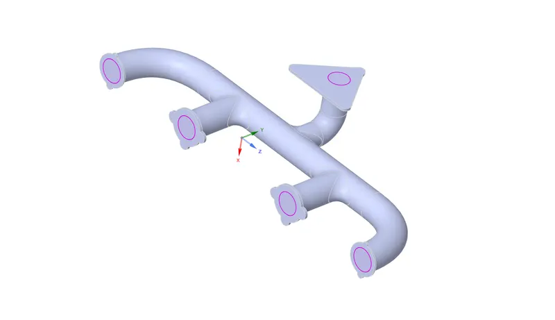
- Import the geometry in spaceclaim.
- Firstly, check for the duplicate edges, if any edges found clear them.
- Then we extract the fluid volume by the volume extract option.
- Renaming and moving them to a single head 'final geometry'
- Then we enable the share topology option. This option helps to transfer information from body to another body. In this case it is between solid volume and fluid volume
Meshing :
Name sections :
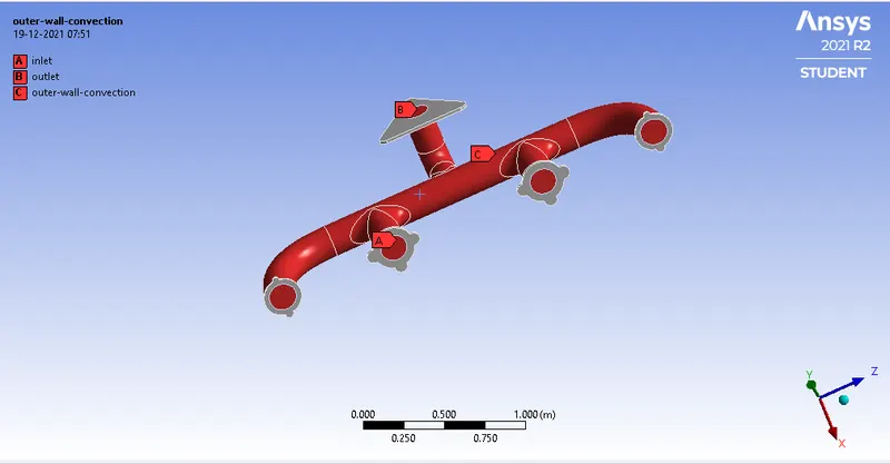
CASE 1 :
A] Pre-Processing :
| Turbulence model | K-epsilon (Standard) |
| Wall functions | Standard wall functions |
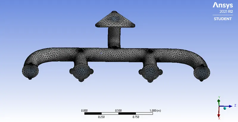
1.1 Mesh Details :
| Element Size | 150 mm | --- |
| Total number of cells | 1,36472 | Coarse |
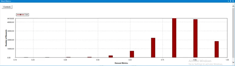
Mesh quality :
SETUP AND RESULTS :
|
SETUP |
||
|
Solver Type |
Pressure-Based |
|
|
Velocity Formulation |
Absolute |
|
|
Time |
|
|
|
Viscous Model |
K-epsilon | |
|
Material |
Fluid type: Air Solid-type: Aluminium |
|
|
Cell zones |
Fluid type: Air Solid-type: Aluminium |
|
|
Boundaries |
Inlet (velocity inlet) Velocity Magnitude 5m/s Temperature – 700K Outlet x (Pressure outlet) Gauge Pressure – 0 pas. Outer-wall-convection -Wall with the thermal condition being convection and heat transfer coefficient All other walls - adiabatic |
|
|
Reference values |
Area = 0.02167`m^2` Length = 0.1661m Density = 1.225kg/`m^3` Enthalpy = 0 J/kg Pressure = 0 pa Temperature = 300K Velocity = 5m/s Viscoity = 1.7894e-05 kg/ms |
b] Post-Processing Results :
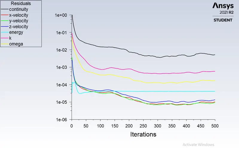
1. Residuals :
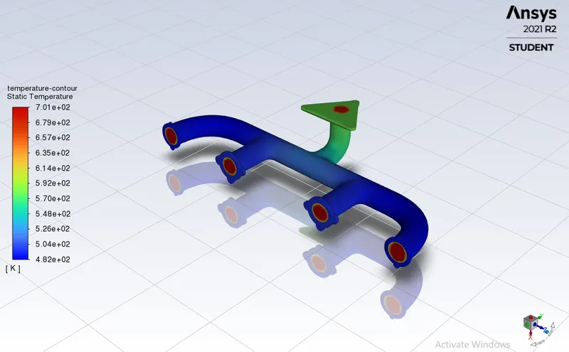
2.1. Temperature Contour :
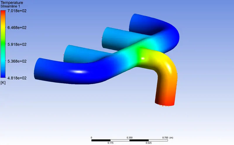
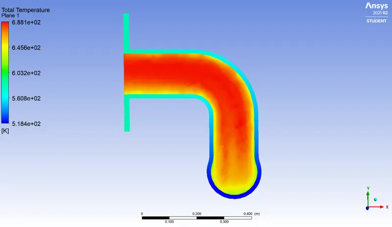
2.2. Temperature :
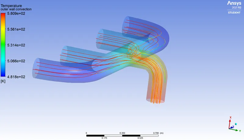
2.3 Temperature streamlines :
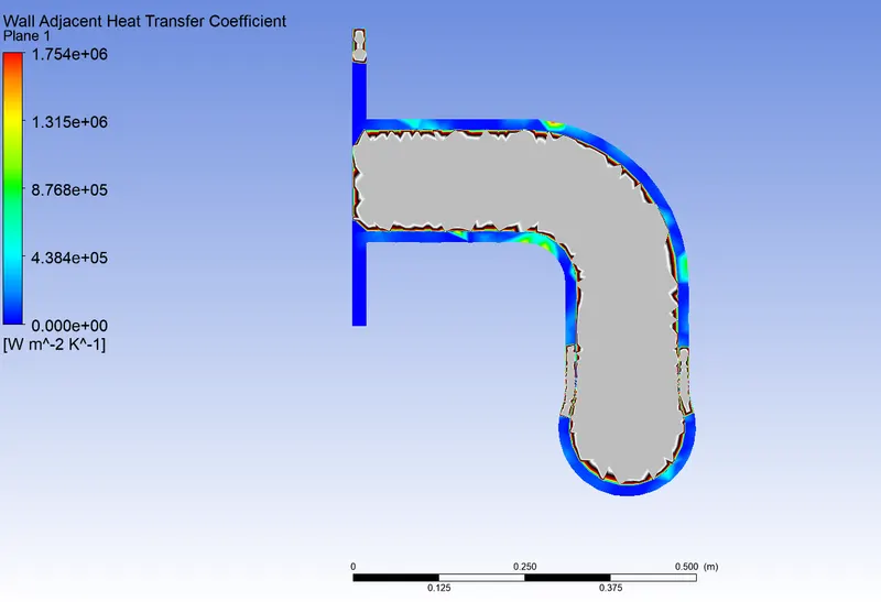
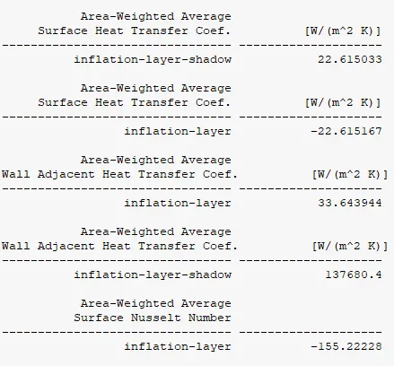
3.1. Wall Adjacent Heat Transfer Coefficient :
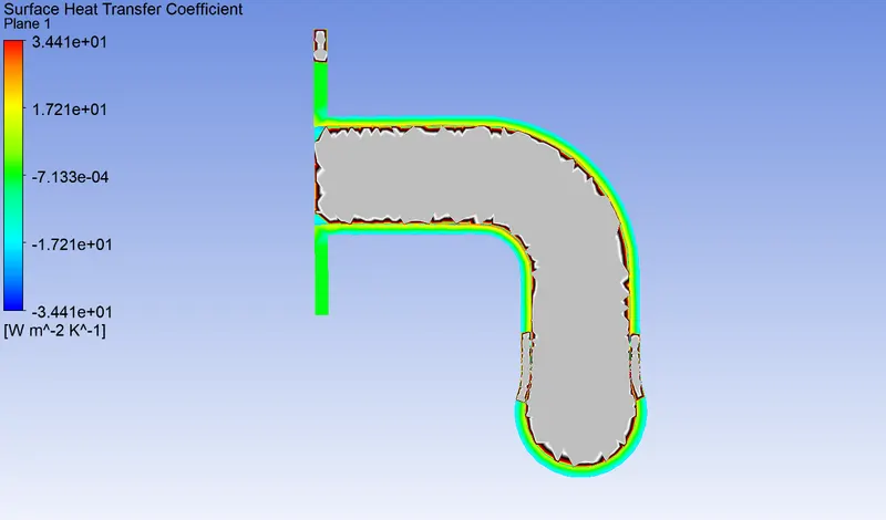
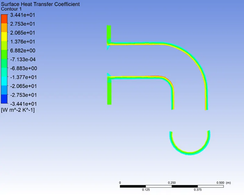
4. Surface Heat Transfer Coefficient :
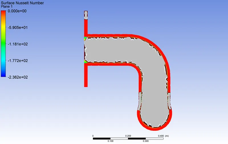
5. Surface Nusselt Number :
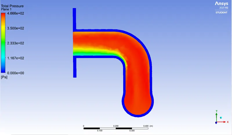
6. Pressure :
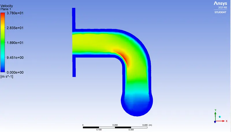
7. Velocity :
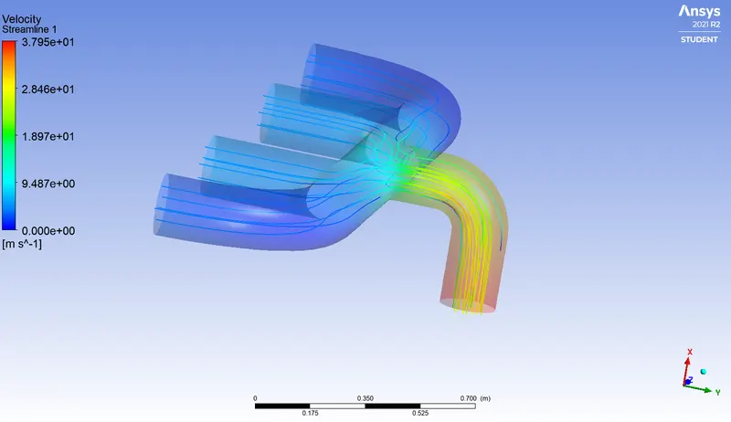
7.1 Velocity streamlines :
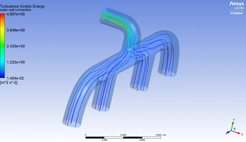
8. Turbulence Kinetic Energy :
c] Post-Processing Reports :
CASE 2 :
| Y+ | 30 |
| Turbulence model | K-epsilon (Standard) |
| Wall functions | Standard wall functions |
A] Pre-Processing :
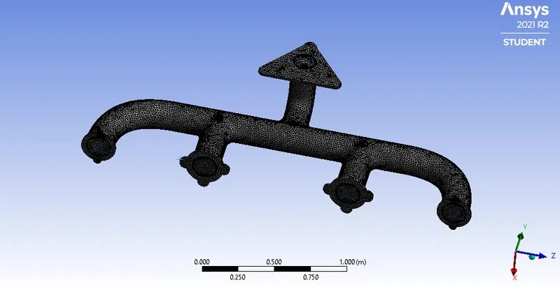
1.1 Mesh Details :
| Element size | 15 mm | -- |
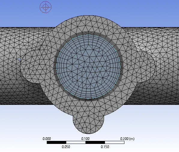
| Number of inflation layers | 5 | -- |
| Growth rate | 1.2 | -- |
| Inflation type | Total thickness | 26 mm |
| Total number of cells | 4,47101 | Refined |
1.2 Mesh :
1.3. Inflation layers in between fluid-solid interaction :
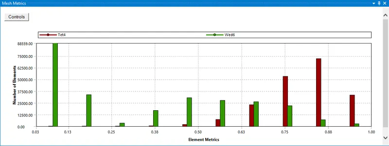
Mesh quality :
SETUP AND RESULTS :
|
SETUP |
||
|
Solver Type |
Pressure-Based |
|
|
Velocity Formulation |
Absolute |
|
|
Time |
|
|
|
Viscous Model |
K-epsilon | |
|
Material |
Fluid type: Air Solid-type: Aluminium |
|
|
Cell zones |
Fluid type: Air Solid-type: Aluminium |
|
|
Boundaries |
Inlet (velocity inlet) Velocity Magnitude 5m/s Temperature – 700K Outlet x (Pressure outlet) Gauge Pressure – 0 pas. Outer-wall-convection -Wall with the thermal condition being convection and heat transfer coefficient All other walls - adiabatic |
|
|
Reference values |
Area = 0.02167`m^2` Length = 0.1661m Density = 1.225kg/`m^3` Enthalpy = 0 J/kg Pressure = 0 pa Temperature = 687K Velocity = 5m/s Viscoity = 1.7894e-05 kg/ms |
b] Post-Processing Results :
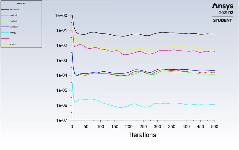
1. Residuals :
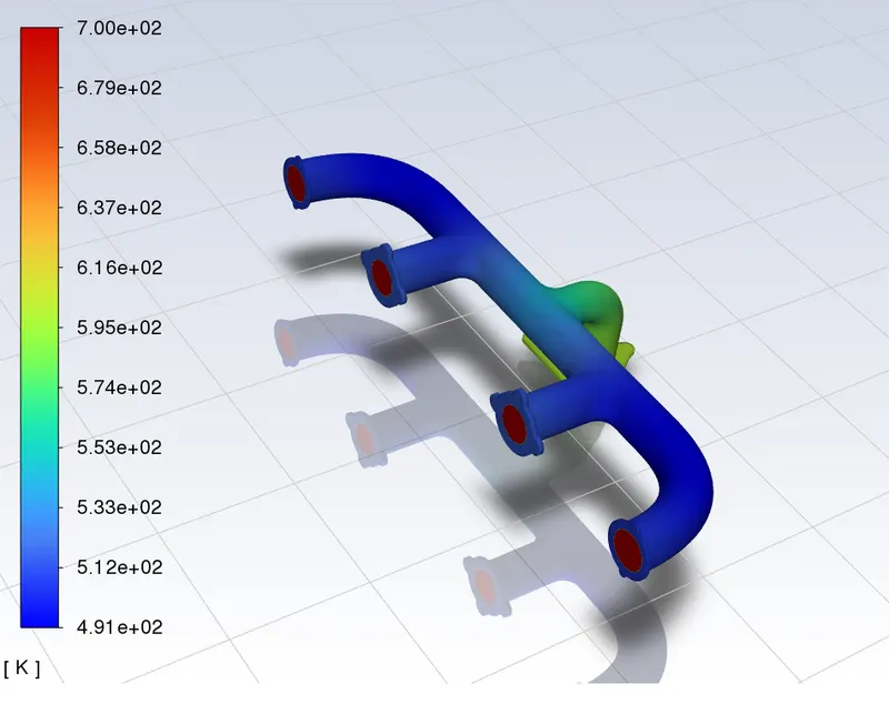
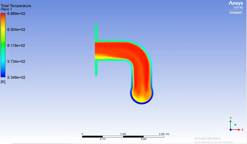
2.1. Temperature Contour :
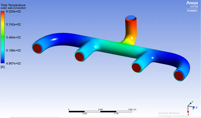
2.2. Temperature :
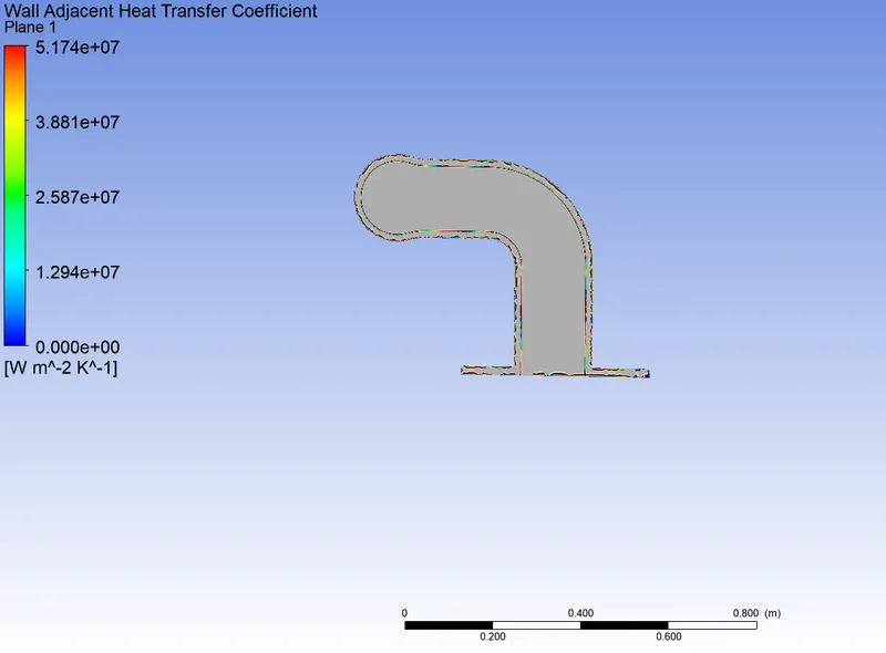
3.1. Wall Adjacent Heat Transfer Coefficient :
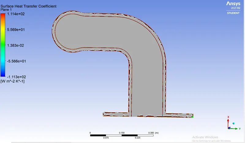
4. Surface Heat Transfer Coefficient :
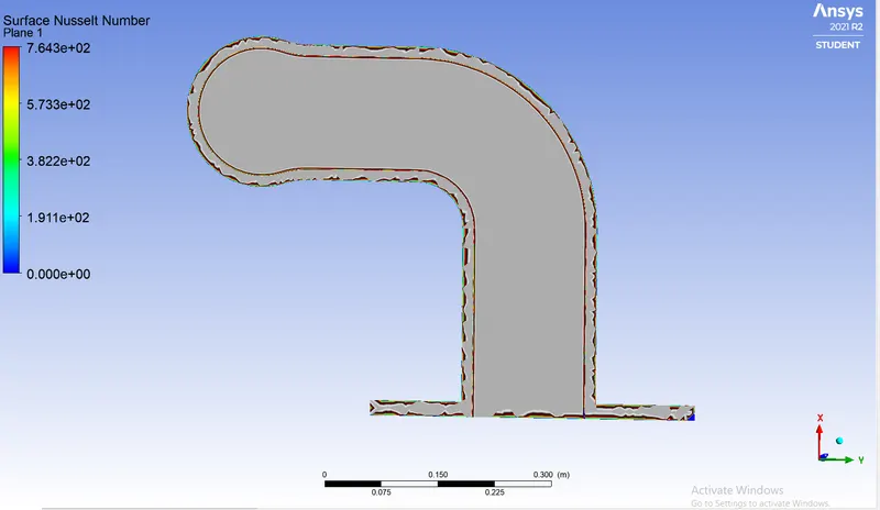
5. Surface Nusselt Number :
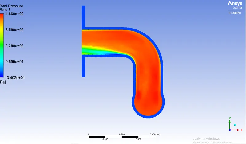
6. Pressure :
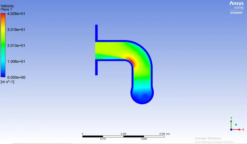
7. Velocity :
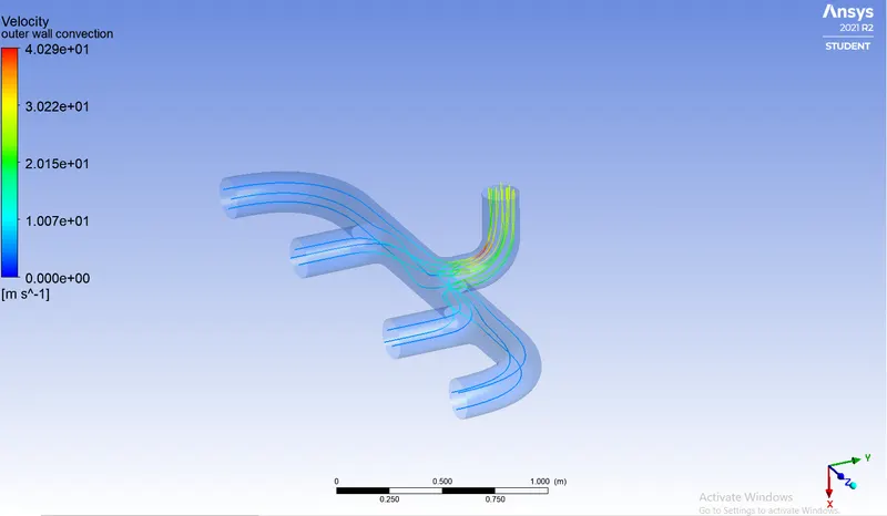
7.2 velocity streamlines :
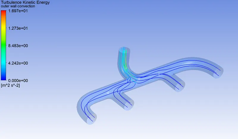
8. Turbulence Kinetic Energy :
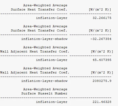
C] Post-Processing Reports :
CASE 3 :
| Y+ | 5 |
| Turbulence model | K-omega (SST) |
A] Pre-Processing :
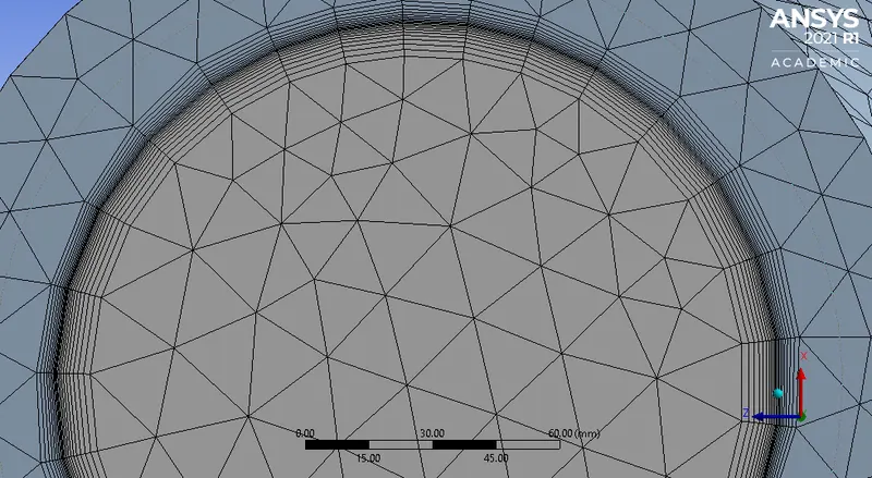
1.1. Mesh Details :
| Element size | 17 | -- |
| Number of inflation layers | 7 | -- |
| Growth rate | 1.2 | -- |
| Inflation type | Total thickness | 8 mm |
| Total number of cells | 492888 | Refined |
1.2 Mesh :
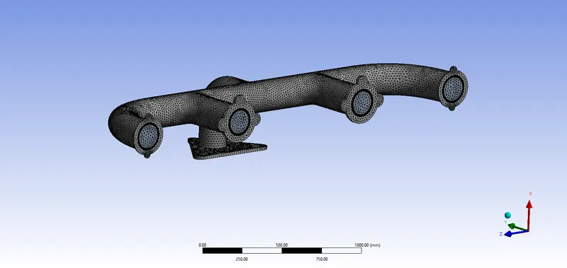
1.3. Inflation layer in between fluid-solid interaction :
SETUP AND RESULTS :
|
SETUP |
||
|
Solver Type |
Pressure-Based |
|
|
Velocity Formulation |
Absolute |
|
|
Time |
|
|
|
Viscous Model |
K-omega | |
|
Material |
Fluid type: Air Solid-type: Aluminium |
|
|
Cell zones |
Fluid type: Air Solid-type: Aluminium |
|
|
Boundaries |
Inlet (velocity inlet) Velocity Magnitude 5m/s Temperature – 700K Outlet x (Pressure outlet) Gauge Pressure – 0 pas. Outer-wall-convection -Wall with the thermal condition being convection and heat transfer coefficient All other walls - adiabatic |
|
|
Reference values |
Area = 0.02167`m^2` Length = 0.1661m Density = 1.225kg/`m^3` Enthalpy = 0 J/kg Pressure = 0 pa Temperature = 687K Velocity = 5m/s Viscoity = 1.7894e-05 kg/ms |
b] Post-Processing Results :
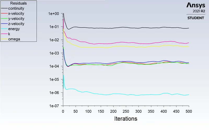
1. Residuals :
2.1. Temperature Contour :
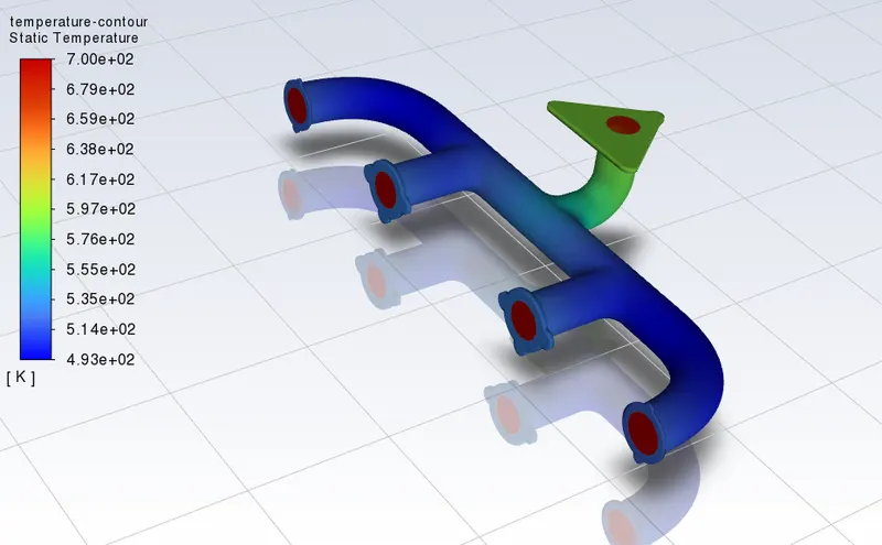
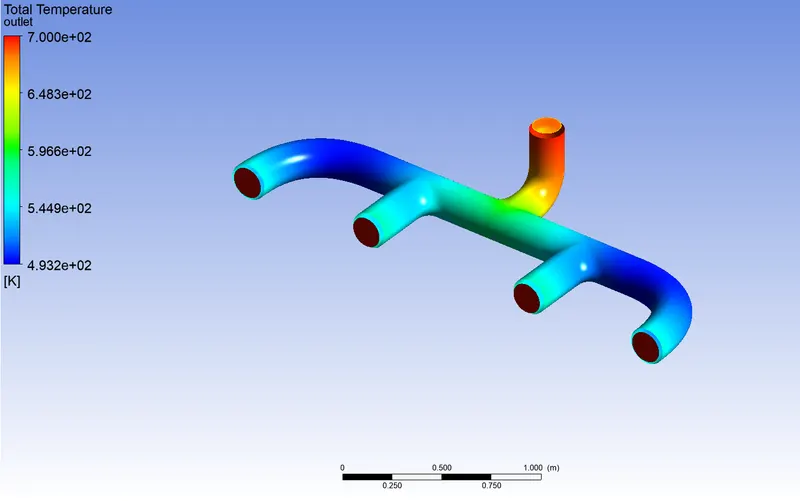
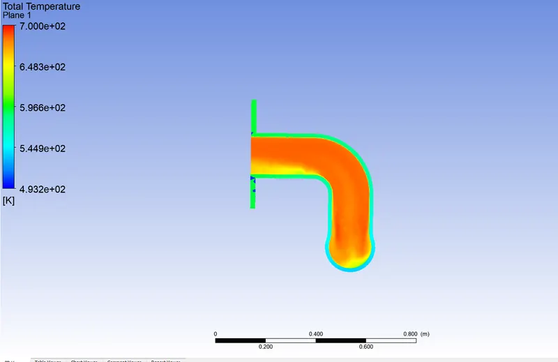
2.2. Temperature :
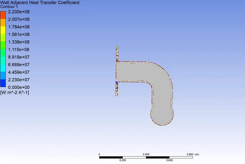
3.1. Wall Adjacent Heat Transfer Coefficient :
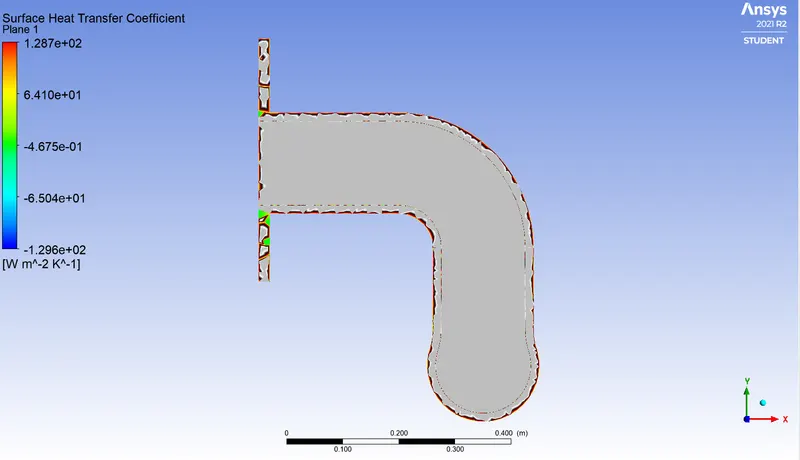
4. Surface Heat Transfer Coefficient :
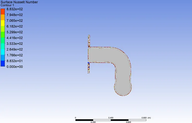
5. Surface Nusselt Number :
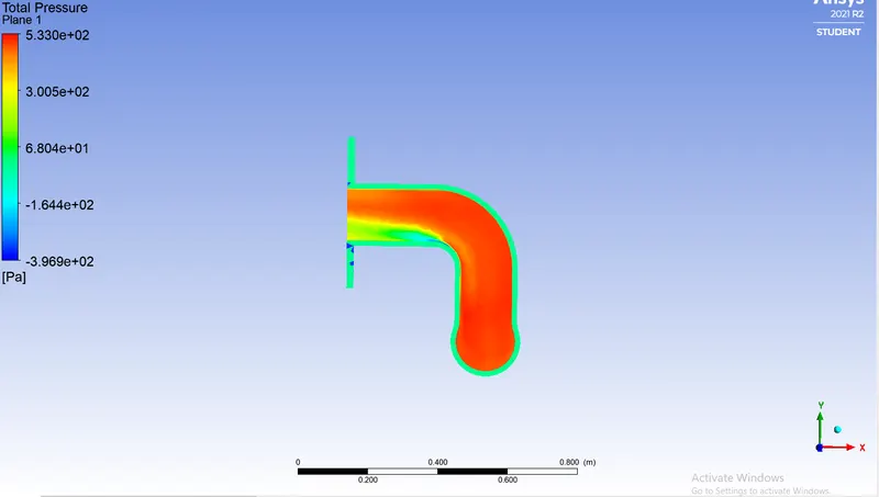
6. Pressure :
7. Velocity :
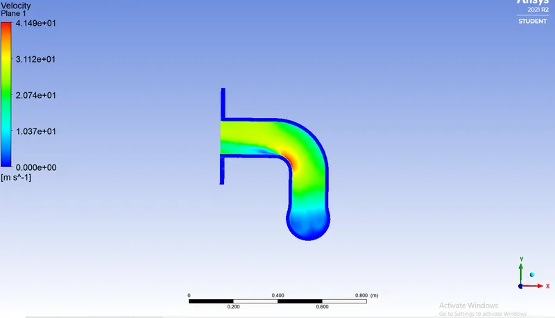
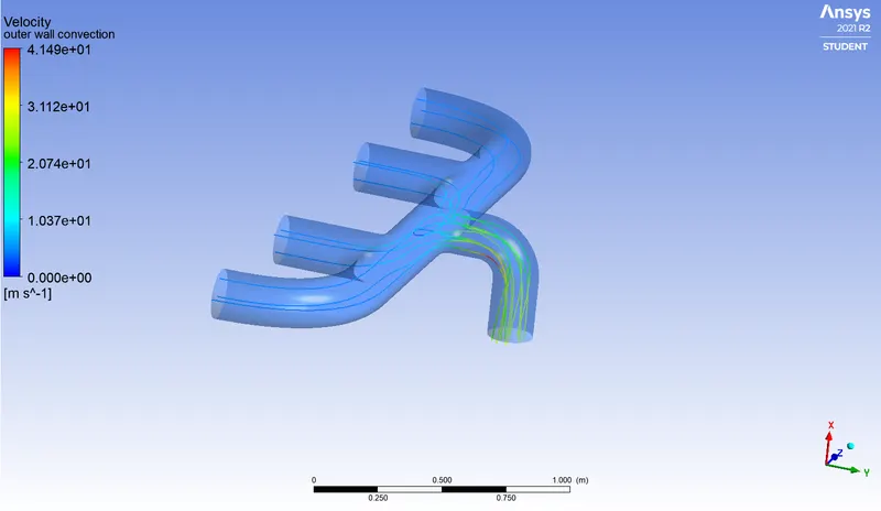
7.2 Velocity streamlines :
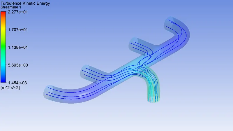
8. Turbulence Kinetic Energy :
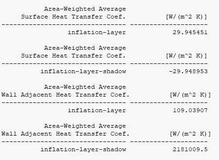
C] Post-Processing Reports :

Note :
- Wall adjacent heat transfer coefficient uses difference of wall temperature and temperature of cell adjacent to the wall.
Wall adjacent heat transfer coefficient = wall heat flux/ (wall temperature - wall adjacent temperature)
- Surface heat transfer coefficient uses difference of wall temperature and reference fluid temperature (bulk fluid temperature).
Surface heat transfer coefficient = wall heat flux / (wall temperature - bulk fluid temperature)
How would you verify if the HTC predictions from the simulations are right?
- The heat transfer coefficient can be verified by comparing the values analytically.
- Analytically heat transfer coefficient can be calculated with the help of Dittus-Boelter equation,
`Nu = 0.023Re^0.8Pr^0.4` (when fluid is heated along with the flow)
And `Nu = 0.023Re^0.8Pr^0.3` (When fluid is cooled along with the flow)
- In this case, heated fluid is loosing heat (thermal energy) to the walls of the manifold.
- So, `Nu= 0.023Re^0.8Pr^0.3` is used to calculate the Nusselt number of the respective case.
- Finally the heat transfer coefficient is calculated usimh nusselt number(Nu) = `(hL)/(k)`
h = Heat transfer coefficient `(W)/(m^2K)`
D_h = hydraulic diameter (m)
K = Thermal conductivity of the fluid`(W)/(mK)`
Note: The heat transfer coefficient obtained using analytical means is calculated using the bulk fluid temperature and not with the local wall adjacent temperatures. For numerical validation it is required to take surface heat transfer coefficient in place of wall adjacent heat transfer coeffcient / wall function heat transfer coefficient.
We know that Nusselt no and reynold no are directly propotional and reynold no is proportional to velocity. So HTC is directly proportional to velocity. And from the contours we can see that velocity and HTC are highest at the outlet. So we can predict the results are correct.
What factors does the accuracy of the prediction depend on?
1. Mesh size-Finer the mesh better is the results.
2. Adding inflation layer gives better results.
3. Choosing appropriate turbulence model gives better result.
Conclusion :
1. The baseline mesh gave almost accurate results. But finer mesh gave more accurate results.
2. Surface heat transfer coefficient was captured smoothly and more acurately in the case of finer mesh.
3. Wall adjacent heat transfer co-efficent was calculated from each cell center which may lead to incorrect result because HTC is depends on the mesh size. So, this method is not suitable for validating.
3. Adding inflation layer gave better results.
References :
1. https://www.comsol.com/blogs/conjugate-heat-transfer/
2. https://www.afs.enea.it/project/neptunius/docs/fluent/html/ug/node469.htm
3. ANSYS Fluent user's guide