Week 2 - Flow over a Cylinder.
Aim :
To simulate the flow over a cylinder and explain the phenomenon of Karman vortex street.
Objective :
- To simulate the flow over a cylinder for different cases and explain the phenomenon of Karman vortex street.
- To discuss the effect of Reynolds number on the coefficient of drag. [ Results should be validated with any standard literature and error should be within 5 %]
- To Plot the coefficient of drag and lift.
- Plot to show vortex shedding behind the cylinder.
Cases :
Case 1 :
- Simulate the flow with the steady and unsteady case and calculate the Strouhal Number for Re= 100.
Case 2 :
- Calculate the coefficient of drag and lift over a cylinder by setting the Reynolds number to 10,100,1000,10000 & 100000. (Run with steady solver)
- Discuss the effect of Reynolds number on the coefficient of drag. [ Results should be validated with any standard literature and error should be within 5 %]
Theory :
Flow seperation over a cylinder :
For a while forget about the cylinder or the sphere. Consider a thin flat plate kept in a flow. When the flow is passing over the plate, the layer of the fluid just adjacent to the plate surface will obviously experience viscous drag force. The magnitude of this drag experienced by subsequent layers will go on reducing as u start going up from the lowest layer. This gives rise to the formation of the boundary layer.
If its a cylinder/sphere;
The tangential flow speed just outside the boundary layer (neglecting any circulation of the external flow around the cylinder) is
`U(theta) = 2Uosintheta`
- By Bernoulli's principle, In the front part as speed is increasing along the flow direction, pressure is reducing. this is called favorable pressure gradient.(because, flow tends to occur always from high pressure to low pressure)
- But, on the other side of the sphere or cylinder, the speed is reducing, it means, the pressure is increasing along the flow.clearly this if an adverse pressure gradient. as, the flow is now tending to flow backwards(due to the positive pressure gradient).
- Now in this situation at some point the flow will appear to be stopped.(actual forward flow and tendency to flow backwards are equal ). this exactly, is the point of separation. here onward, the forward flow will no more stick to the surface and hence the boundary layer separation occurs.
Strouhal number :
The Strouhal Number can be important when analyzing unsteady, oscillating flow problems. The Strouhal Number represents a measure of the ratio of the inertial forces due to the unsteadiness of the flow or local acceleration to the inertial forces due to changes in velocity from one point to an other in the flow field.
- For large strouhal number (order of 1), viscosity dominates fluid slow, resulting in a collective oscillating movement of the fluid ''plug''.
- For low strouhal number (order of `10^-4` and below), the high-speed, quasi-steady-state portion of the movement dominates the oscillation.
- Oscillation at intermediate strouhal number is characterized by the buildup and rapidly subsequent shedding of vortices.
`S = (omegaD)/(U)`
Where as,
`omega` - frequency of vortex shedding.
D - Characteristic diameter of the cylinder.
U - fluid flow velocity.
Co-efficient of drag :
Its a dimensionless quantity that is used to quantify the drag or resistance of an object in a fluid environment, such as air or water. It is used in the drag equation in which a lower drag coefficient indicates the object will have less aerodynamic or hydrodynamic drag. The drag coefficient is always associated with a particular surface area.
`C_d = (2F)/(ρAV^2)`
F - Drag force.
`C_d` - Drag coefficient.
`rho` - Density of fluid.
A - Area of the object facing the fluid.
V - Velocity of the fluid.
`C_d` contains all the complex dependencies and it is usually determine experimentally. Choice of area A affects the value of `C_d`.
Co-efficient of lift :
The lift coefficient is a number that aerodynamicists use to model all of the complex dependencies of shape, inclination, and some flow conditions on lift. This equation is simply a rearrangement of the lift equation where we solve for the lift coefficient in terms of the other variables. The lift coefficient Cl is equal to the lift L divided by the quantity: density r times half the velocity V squared times the wing area A.
`Cl = L / (A * .5 * r * V^2)`
The quantity one half the density times the velocity squared is called the dynamic pressure q. So
`Cl = L / (q * A)`
The lift coefficient then expresses the ratio of the lift force to the force produced by the dynamic pressure times the area.
Solution and Result :
Solving a flow over a cylinder
1. Geometry :
Computational Domain :
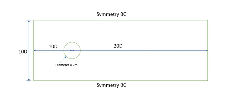

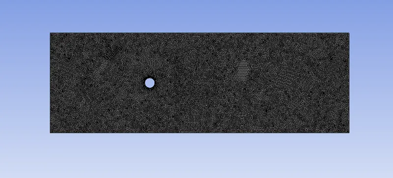
2. Meshing :
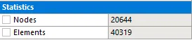
Number of elements and nodes :
- In meshing triangular method is used with an element size of 0.25
- For further refinement of a circle which is the walls of a cylinder sizing command is used and in that select cylinder edge to be refined and gave number of divisions = 48. Now the cylinder is much more refined.
- In order to capture physics effectivey body fitted mesh is used. For that provide inflation layer in the area where we needed to capture physics accurately. So provide 6 inflation layer and in inflation option choose first layer thickness and provide a thickness of 5e-3.
Solution :
Case 1 :
Subcase 1 :
Steady state (Reynolds number = 100) :
| Steady state (Reynolds number = 100) | |
| Solver type | pressure-based |
| Velocity formulation | Absolute |
| Time | Steady |
| Viscous model | Laminar |
| Material |
user-defined Viscosity - 0.05 kg m s Density - 1kg/`m^3` |
| cell zones ff_surface | Fluid type : user-defined |
| Boundaries | Inlet x (velocity inlet) |
| velocity magnitude - 2.5m/s | |
| Temperature - standard | |
| Outlet x (pressure outlet) | |
| Gauge pressure - 0pa | |
| Walls - noslip | |
| symmetry - symmetry | |
Residual plot :
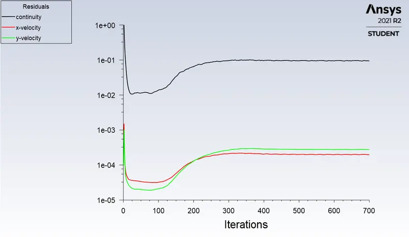
In the above figure residuals are almost equal so the solution is converged.
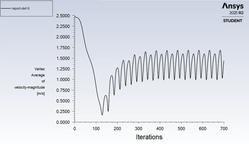
Vertex average of velocity plot :
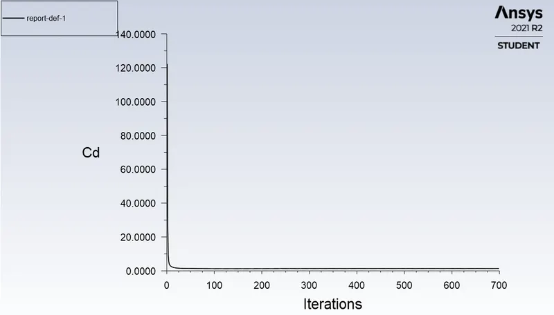
Co-efficient of drag plot:
Co-efficient of drag :

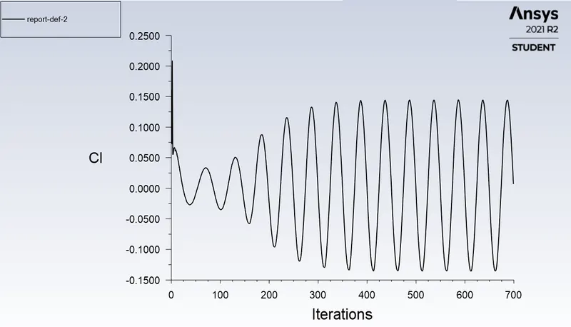
Co-efficient of lift plot :
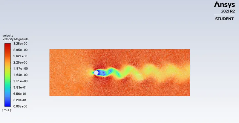
Velocity contour plot :
pressure contour plot :
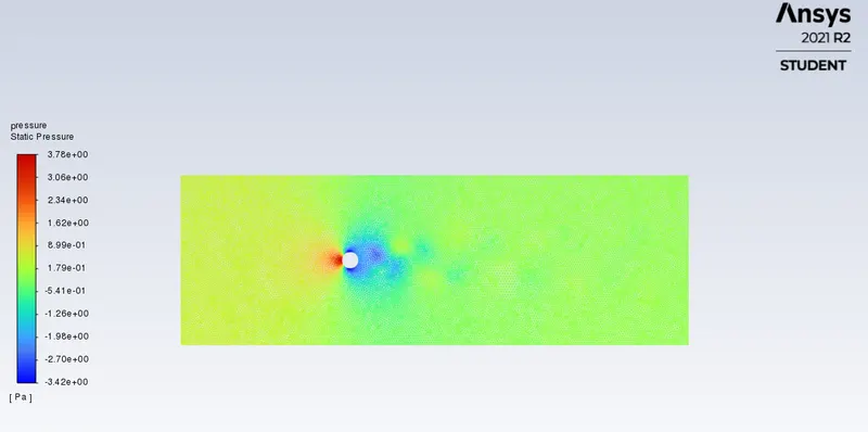
In steady state condition it is not possible to calculate the strouhal number since it is a time dependent.
Subcase 2 :
Unsteady state (Reynolds number = 100) :
| Unsteady state (Reynolds number = 100) | |
| Solver type | pressure-based |
| Velocity formulation | Absolute |
| Time | Unsteady |
| Viscous model | Laminar |
| Material |
user-defined Viscosity - 0.05 kg m s Density - 1kg/`m^3` |
| cell zones ff_surface | Fluid type : user-defined |
| Boundaries | Inlet x (velocity inlet) |
| velocity magnitude - 2.5m/s | |
| Temperature - standard | |
| Outlet x (pressure outlet) | |
| Gauge pressure - 0pa | |
| Walls - noslip | |
| symmetry - symmetry | |
Residual plot :
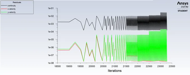
In the above figure residuals are fluctuating about its mean value so the solution is converged.
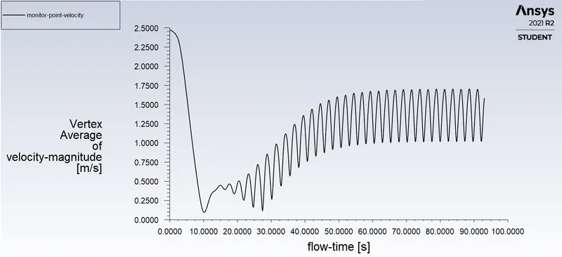
Vertex average of velocity plot :
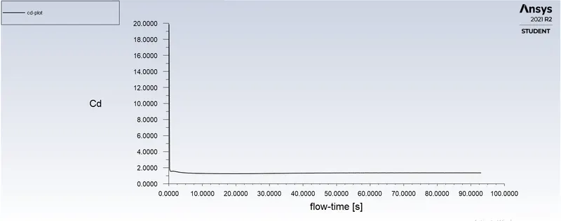
Co-efficient of drag plot:
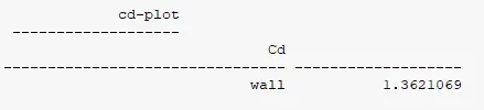
Co-efficient of drag :
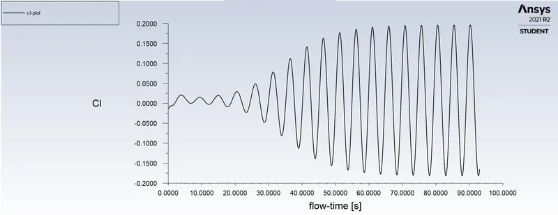
Co-efficient of lift plot :
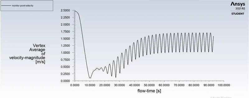
Velocity contour plot :
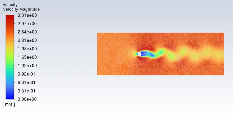
velocity contour plot :
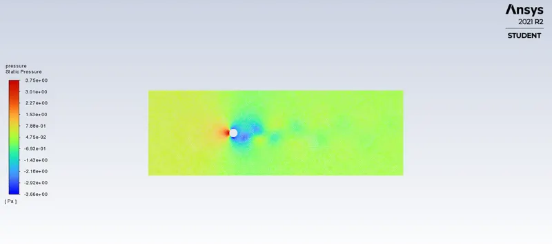
pressure contour plot :
Strouhal number :
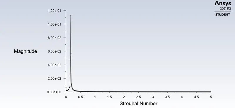
| Numerical strouhal number | Analytical strouhal number |
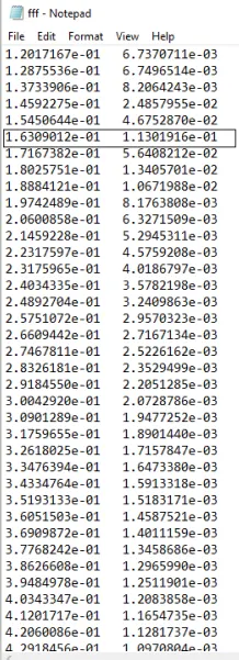 |
`S = (omegaD)/(U')` `omega` = No. of oscillations/Time difference `omega = 2/10` = 0.2 S = `(0.2xx2)/(2.5)` = 0.16 |
From the above table it is clear that the analytically calculated strouhal number equals the numerical strouhal number. Thus it is verfied.
Comparison of drag co-efficent for reynolds number 100 :
| Condition | Analytical value | Numerical value | Error(%) |
| Steady state | 1.347501 | 1.3644105 | 1.25 |
| Unsteady state | 1.3621069 | 1.0839 |
From the above table it is clear that numerical value closely matches the analytical value and the error is within 5% for both the cases.
Case 2 :
Steady state simulation for Reynolds number 10,100,1000,10000 & 100000.
Subcase 1 :
Steady state (Reynolds number = 10) :
| Steady state (Reynolds number = 10) | |
| Solver type | pressure-based |
| Velocity formulation | Absolute |
| Time | Steady |
| Viscous model | Laminar |
| Material |
user-defined Viscosity - 0.05 kg m s Density - 1kg/`m^3` |
| cell zones ff_surface | Fluid type : user-defined |
| Boundaries | Inlet x (velocity inlet) |
| velocity magnitude - 0.25m/s | |
| Temperature - standard | |
| Outlet x (pressure outlet) | |
| Gauge pressure - 0pa | |
| Walls - noslip | |
| symmetry - symmetry | |
Residual plot :
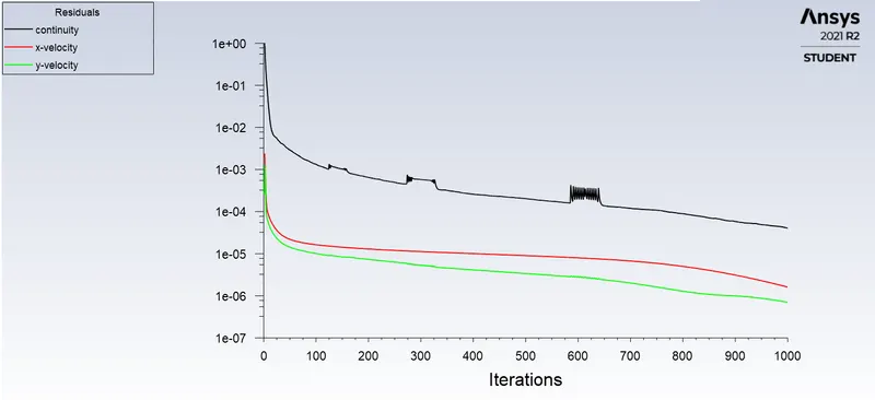
In the above figure the residuals are converged below 1e-5 so the solution is converged.
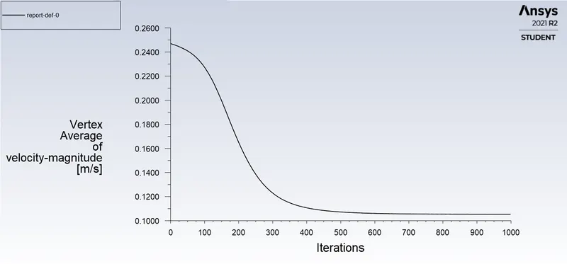
Vertex average of velocity plot :
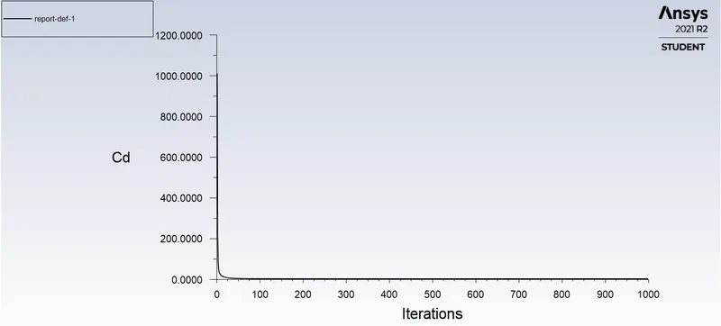
Co-efficient of drag plot :
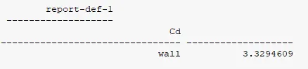
Co-efficient of drag :
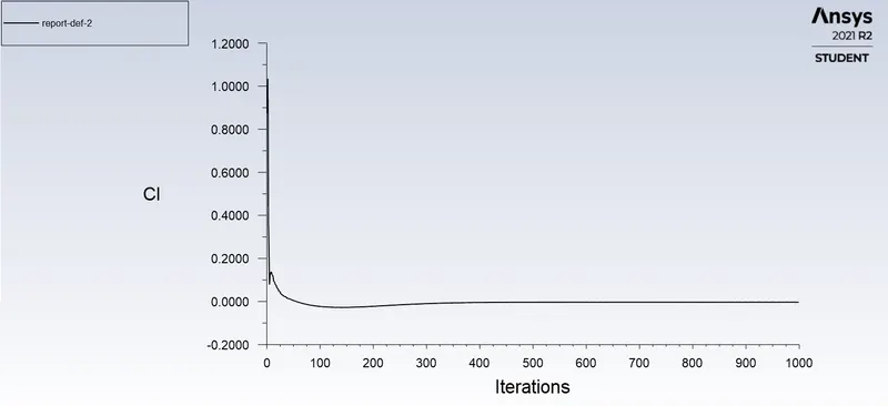
Co-efficient of lift plot :
Velocity contour plot :
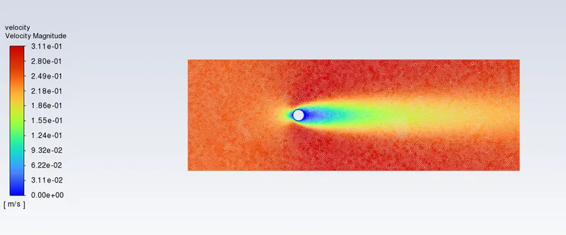
pressure contour plot :
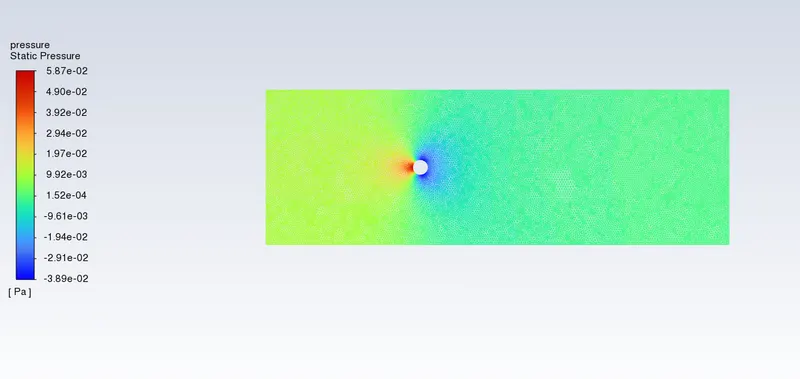
Subcase 2 :
Steady state (Reynolds number = 100) :
| Steady state (Reynolds number = 100) | |
| Solver type | pressure-based |
| Velocity formulation | Absolute |
| Time | Steady |
| Viscous model | Laminar |
| Material |
user-defined Viscosity - 0.05 kg m s Density - 1kg/`m^3` |
| cell zones ff_surface | Fluid type : user-defined |
| Boundaries | Inlet x (velocity inlet) |
| velocity magnitude - 2.5m/s | |
| Temperature - standard | |
| Outlet x (pressure outlet) | |
| Gauge pressure - 0pa | |
| Walls - noslip | |
| symmetry - symmetry | |
Residual plot :
In the above figure residuals are almost equal so the solution is converged.
Vertex average of velocity plot :
Co-efficient of drag plot:
Co-efficient of drag :
Co-efficient of lift plot :
Velocity contour plot :
pressure contour plot :
Subcase 3 :
Steady state (Reynolds number = 1000) :
Mesh is made much finer in order to capture the physics effectively.
Meshing :
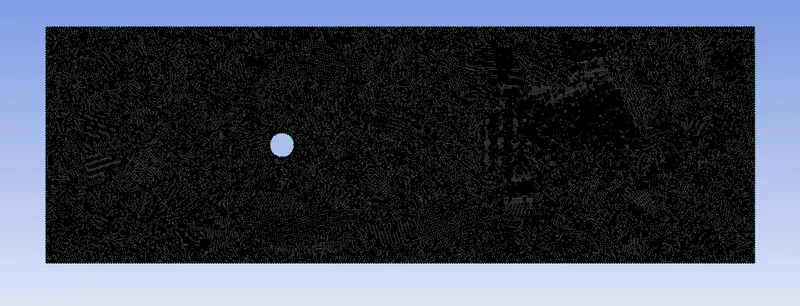
In meshing triangular method is used with an element size of 0.1m.
Number of elements and nodes :
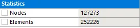
| Steady state (Reynolds number = 1000) | |
| Solver type | pressure-based |
| Velocity formulation | Absolute |
| Time | Steady |
| Viscous model | Laminar |
| Material |
user-defined Viscosity - 0.05 kg m s Density - 1kg/`m^3` |
| cell zones ff_surface | Fluid type : user-defined |
| Boundaries | Inlet x (velocity inlet) |
| velocity magnitude - 25m/s | |
| Temperature - standard | |
| Outlet x (pressure outlet) | |
| Gauge pressure - 0pa | |
| Walls - noslip | |
| symmetry - symmetry | |
Residual plot :
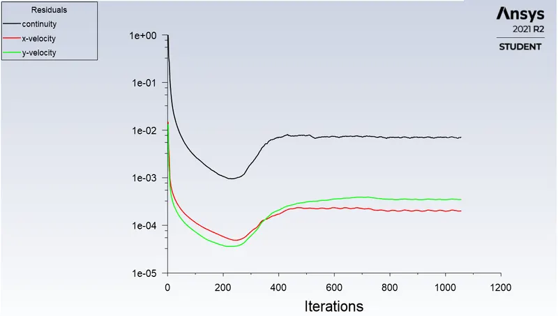
In the above figure residuals are fluctuating about its mean value so the solution is taken converged.
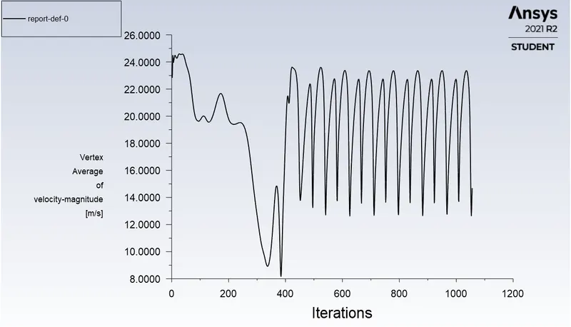
Vertex average of velocity plot :
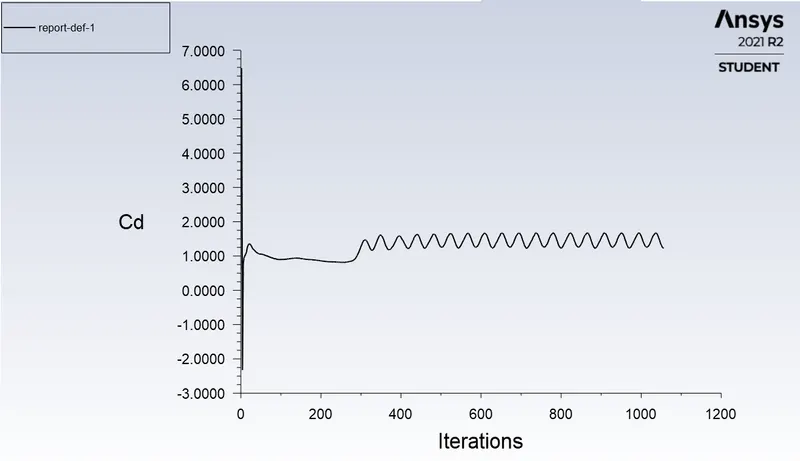
Co-efficient of drag plot :
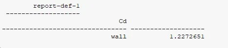
Co-efficient of drag :
Co-efficient of lift plot :
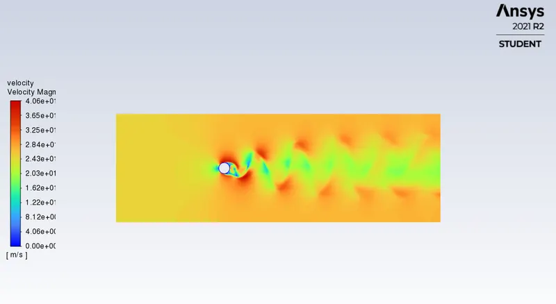
Velocity contour plot :
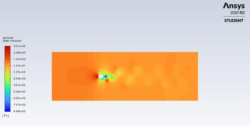
pressure contour plot :
Subcase 4 :
Steady state (Reynolds number = 10000) :
Here mesh is further refined in order to capture the physics efficiently.
Mesh :
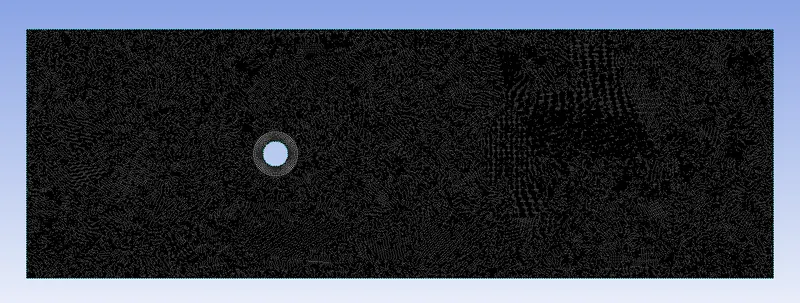
Number of elements and nodes :
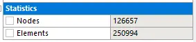
| Steady state (Reynolds number = 10000) | |
| Solver type | pressure-based |
| Velocity formulation | Absolute |
| Time | Steady |
| Viscous model | Laminar |
| Material |
user-defined Viscosity - 0.05 kg m s Density - 1kg/`m^3` |
| cell zones ff_surface | Fluid type : user-defined |
| Boundaries | Inlet x (velocity inlet) |
| velocity magnitude - 250m/s | |
| Temperature - standard | |
| Outlet x (pressure outlet) | |
| Gauge pressure - 0pa | |
| Walls - noslip | |
| symmetry - symmetry | |
Residual plot :
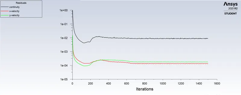
In the above figure residuals are fluctuating about its mean value so the solution is taken converged.
Vertex average of velocity plot :
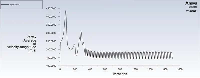
Co-efficient of drag plot:
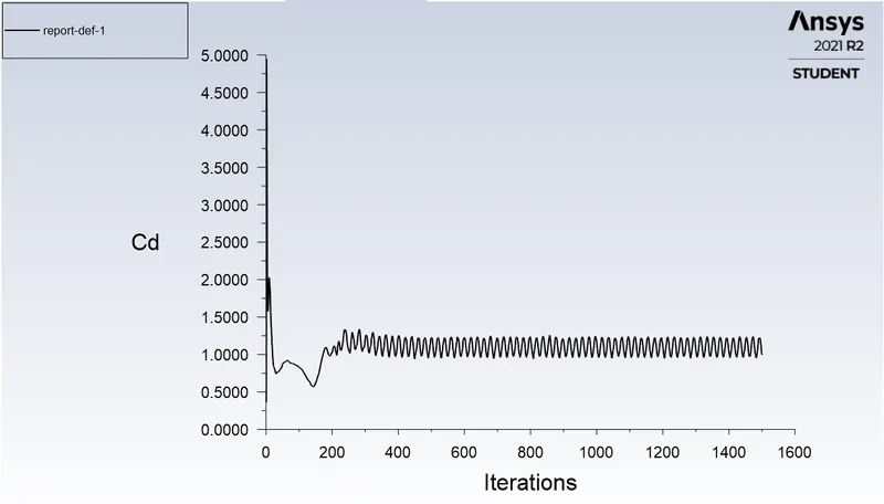
Co-efficient of drag :

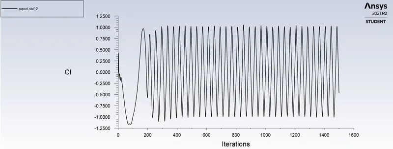
Co-efficient of lift plot :
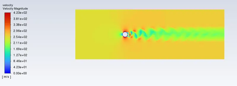
Velocity contour plot :
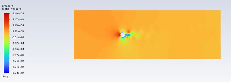
pressure contour plot :
Subcase 5 :
Steady state (Reynolds number = 100000) :
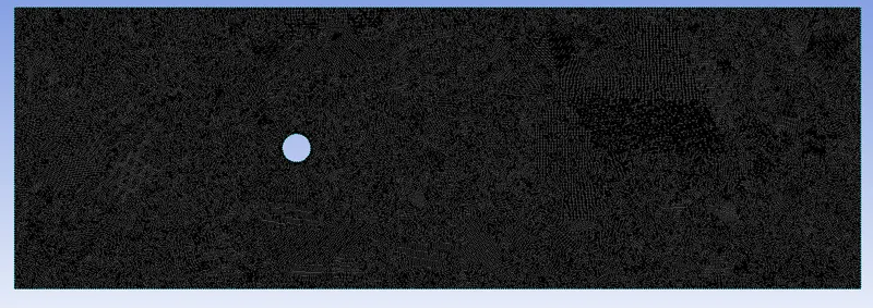
Here the mesh is further refined in order to capture the physics efficiently.
Mesh :
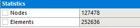
Number of elements and nodes :
| Steady state (Reynolds number = 100000) | |
| Solver type | pressure-based |
| Velocity formulation | Absolute |
| Time | Steady |
| Viscous model | Laminar |
| Material |
user-defined Viscosity - 0.05 kg m s Density - 1kg/`m^3` |
| cell zones ff_surface | Fluid type : user-defined |
| Boundaries | Inlet x (velocity inlet) |
| velocity magnitude - 2500m/s | |
| Temperature - standard | |
| Outlet x (pressure outlet) | |
| Gauge pressure - 0pa | |
| Walls - noslip | |
| symmetry - symmetry | |
Residual plot :
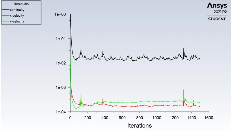
In the above figure residuals are fluctuating about its mean value so the solution is taken converged.
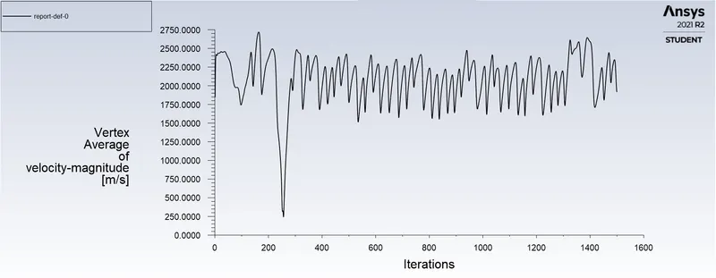
Vertex average of velocity plot :
Co-efficient of drag plot:
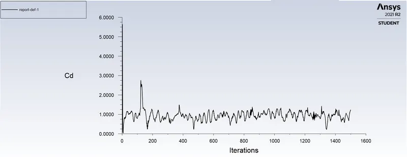
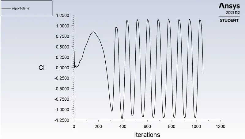
In the above figure we can see that the drag co-efficients are fluctuating about its mean value over the iterations so we can take the mean value of last 20 iterations as our drag co-efficent.
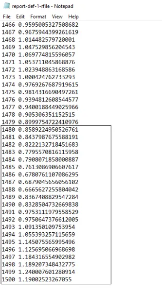
Drag co-efficent(cd) = 0.98245
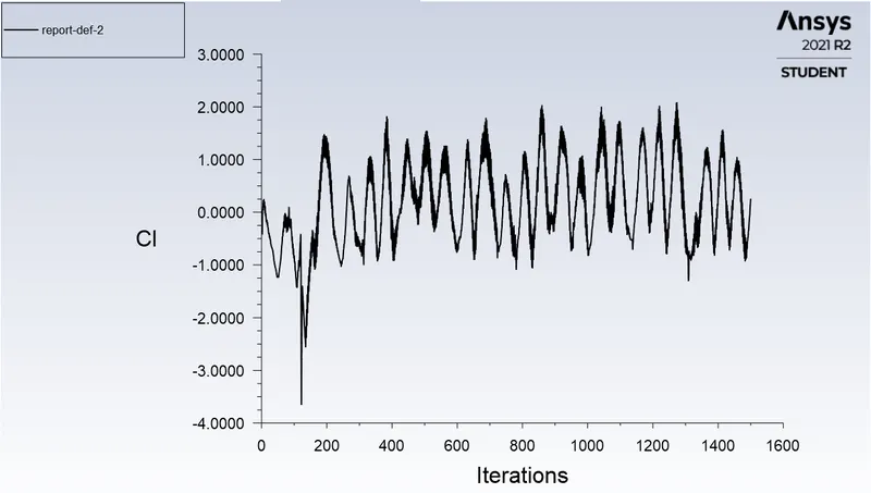
Co-efficient of lift plot :
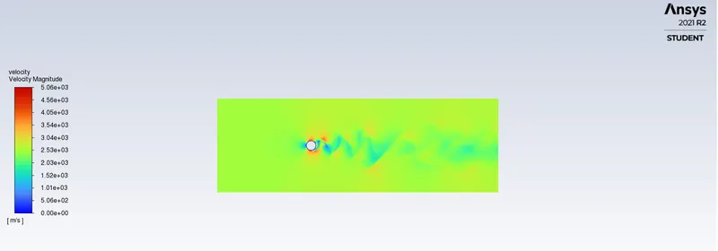
Velocity contour plot :
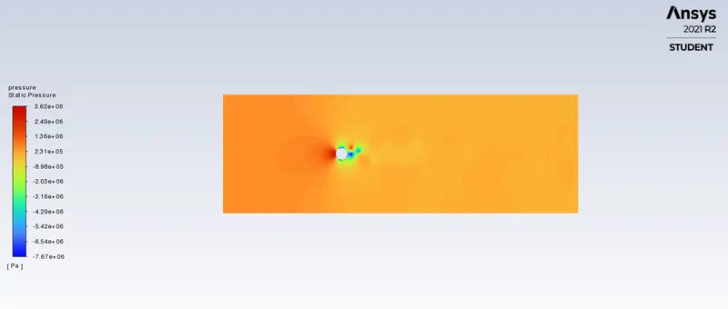
pressure contour plot :
Conclusion :
- Flow over a cylinder is successfully simulated and the effect of phenomena Karman vortex street is successfully analysed for various condition and for the various reynolds number and the result are discussed above.
| Reynolds Number(Re) |
Coefficient of drag(cd) (Analytical value) |
Coefficient of drag(cd) (Numerical value) |
Error(%) |
| 10 | 3.355312 | 3.3294609 | 0.77 |
| 100 | 1.347501 | 1.3644105 | 1.25 |
| 1000 | 1.193902 | 1.2272651 | 2.79 |
| 10000 | 1.028611 | 0.99656377 | 3.12 |
| 100000 | 0.953672 | 0.98245 | 3.017 |
- From the above table we can observe that the drag co-efficient decreases with the increase in the reynolds number. Increase in reynolds number leads to vortex shedding at the the upper and lower side of a cylinder surface.
- Vortex shedding takes place when the reynolds number is greater than or equal to 40(Re>40).
- In reynolds number less than 40 there is no formation of vortices.
- In comparing steady state and unsteady state condition. Unsteady state condition produces accurate results. Since the term vortex karman street is time dependent.
Reference :
https://www.sciencedirect.com/science/article/pii/S0307904X08000243