Week 1- Mixing Tee

Aim :

To simulate a fluid through a mixing tee to calculate the mixing effectiveness of the fluid at two different temperatures at the outlet of the mixing tee.

Objective :

• To set up steady-state simulations to compare the mixing effectiveness when hot inlet temperature is 36⁰C & the Cold inlet is at 19⁰C.
• To use the k-epsilon and k-omega SST model for the first case and based on your judgment use the more suitable model for further cases.
• In a table, compare the following values of cell count, average outlet temperature and number of iterations for convergence from the 2 cases.
• To contour plot velocity and temperature on the cut planes along and across the pipe.
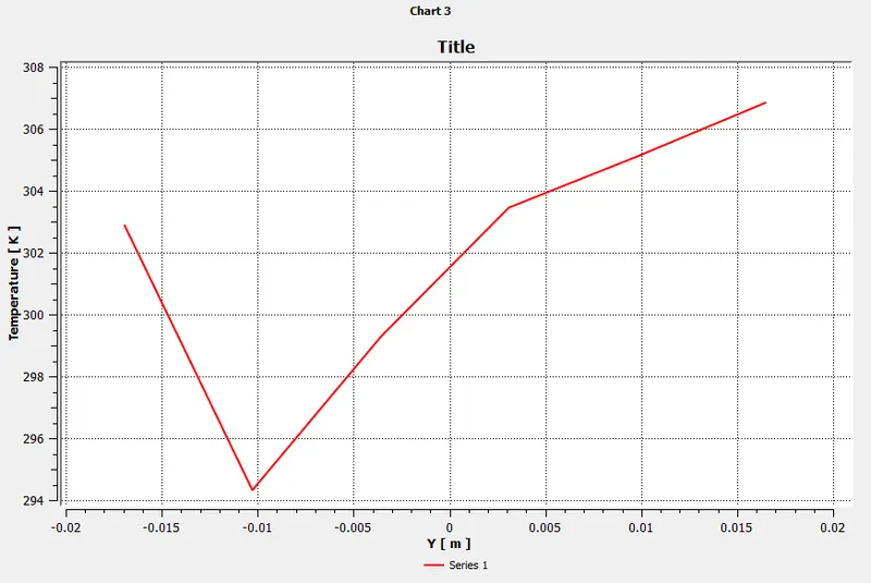
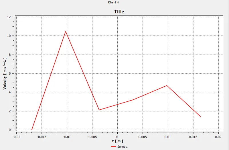
• To line plot velocity and temperature along and across the length of the pipe.
• To perform Mesh independent study for any one case
• To discuss the effect of length and momentum ratio on results.

Problem statement :

1. Case 1
   • Short mixing tee with a hot inlet velocity of 3m/s.
   • Momentum ratio of 2, 4.
2. Case 2
   • Long mixing tee with a hot inlet velocity of 3m/s.
   • Momentum ratio of 2, 4.

Formula :

Momentum ratio = velocity at cold inlet`(V_(cold))` / velocity at hot inlet`(V_(hot))`

`T_(mixture) = ((m_(hot)*T_(hot) +m_(cold)*T_(cold))/(m_(hot)+m_(cold)))`

`m_(hot) = rho_(hot)*A*V_(hot)`

`m_(cold) = rho_(cold)*A*V_(cold)`

Procedure :

Case 1 :

• Short mixing tee with a hot inlet velocity of 3m/s.
• Momentum ratio of 2, 4.

Subcase 1 :

For momentum ratio of 2 :

Momentum ratio = velocity at cold inlet`(V_(cold))` / velocity at hot inlet`(V_(hot))`

2 = `(V_(cold))/3`

`bb(V_(cold))` = 6m/s

Subcase 2 :

For momentum ratio of 4 :

Momentum ratio = velocity at cold inlet`(V_(cold))` / velocity at hot inlet`(V_(hot))`

4 = `(V_(cold))/3`

`bb(V_(cold))` = 12m/s.

Geometry :

Import the step file of the geometry which is the short mixing tee in spaceclaim.

Mesh :

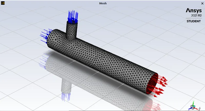
Body meshtype is selected and we have done a mesh refinement for a element size of 0.004. The remain settings are default.

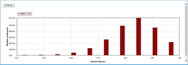
Element mesh quality :

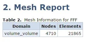
Number of elements and nodes :

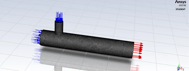
Body meshtype is selected and we have done a mesh refinement for a element size of 0.002. The remain settings are default.

Element mesh quality :

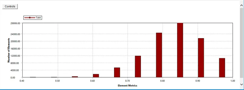
The above graph shows that the mesh quality of each element in that graph it is clear that the mesh quality ranges from minimum to maximum which is greater than 5% so it passes the test.

Number of elements and nodes :

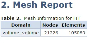
Then we need to name the geometry accordingly

1. Inlet x - Where as the hot air comes in.
2. Inlet y - Where as the cold air comes in.
3. Outlet x - Where the air exits.
4. Walls

Solution :

Short Tee for momentum ratio 2
Setup	k-epsilon	k-omega
Solver type	pressure-based	pressure-based
Velocity formulation	Absolute	Absolute
Time	Steady	Steady
Viscous model	Realizable k-epsilon with standard unction	K-omega SST model
Material	Air	Air
cell zones volume-volume	Fluid type : Air	Fluid type : Air
Boundaries	Inlet x (velocity inlet)	Inlet x (velocity inlet)
	velocity magnitude - 3m/s	velocity magnitude - 3m/s
	Temperature - 36 deg celcius	Temperature - 36 deg celcius
	Inlet y (velocity inlet)	Inlet y (velocity inlet)
	velocity magnitude - 6m/s	velocity magnitude - 6m/s
	Temperature - 19 deg celcius	Temperature - 19 deg celcius
	Outlet x (velocity outlet)	Outlet x (velocity outlet)
	Gauge pressure - 0pa	Gauge pressure - 0pa
	Walls - stationary	Walls - stationary

Results :

Case 1 :

Subcase 1 :

For momentum ratio of 4 which hot air velocity = 3m/s and cold air velocity = 6m/s.

Mesh dependency test :

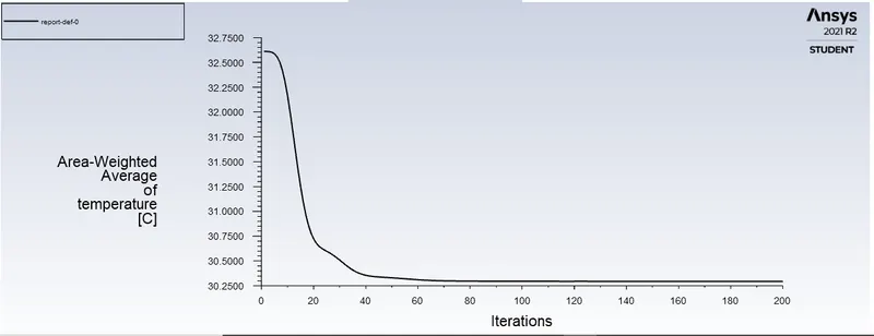
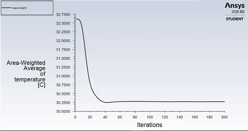
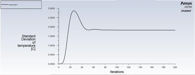
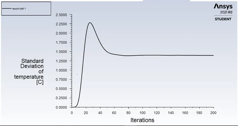
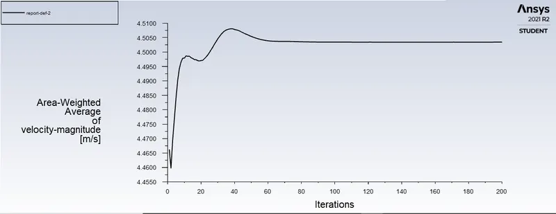
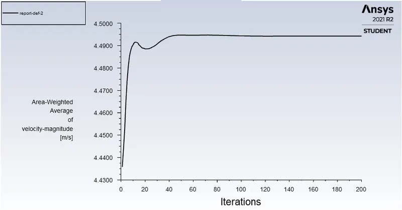
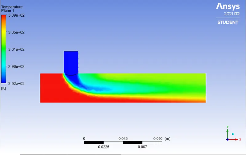
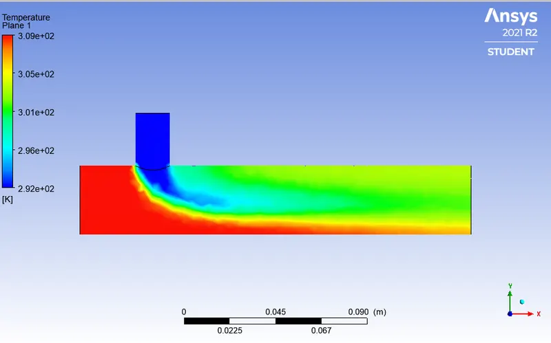
Left being the mesh of element size 0.002 and right being the mesh with a element size of 0.004

Residual plot :

Average weighted area of temperature at the outlet :

Standard deviation of temperature at outlet :

Average weighted area of velocity-magnitude at the outlet :

Contour plot :

1. For temperature distribution :

2. For velocity distribution :

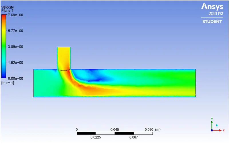
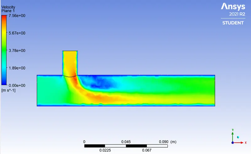
From the above figures it is clear that the mesh with a element size of 0.002 produces a smooth and accurate result than the mesh with a element size of 0.004. From this we can say that mesh with a element size of 0.002 is preffered for further investigation.

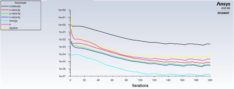
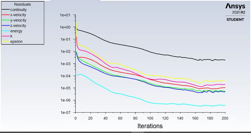
Left being k-epsilon and right being k-omega turbulent model

Residual plot :

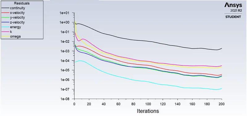
Average weighted area of temperature at the outlet :

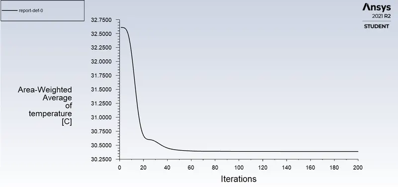
Standard deviation of temperature at outlet :

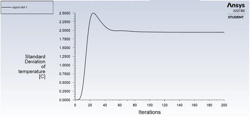
Average weighted area of velocity-magnitude at the outlet :

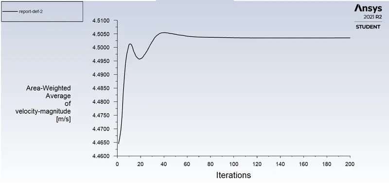
Contour plot :

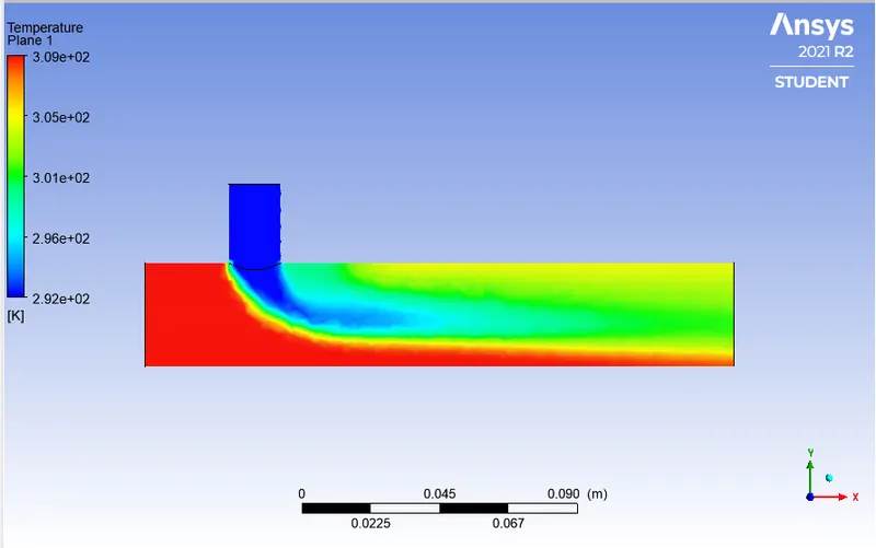
1. For temperature distribution :

2. For velocity distribution :

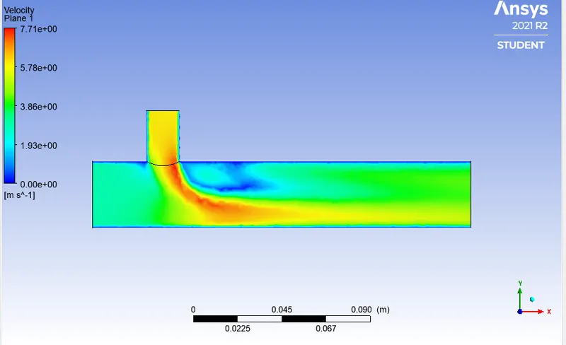
From the above figures it is clear that the k-epsilon turbulence model produces a smooth and accurate result than the k-omega SST model. Since k-omega SST model is generally used to compute solution near the walls, where as k-epsilon model is used to compute solution away from the walls each model has certain advantages. From this we can say that k-epsilon turbulence model is preferred for further investigation.

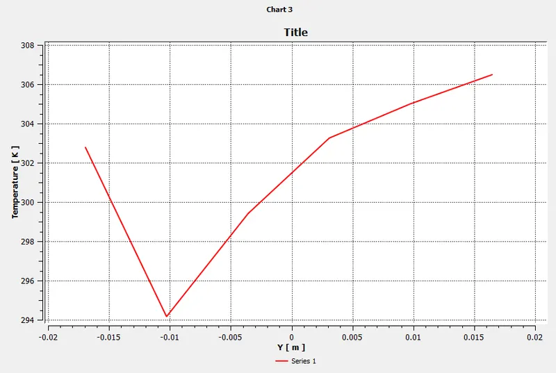
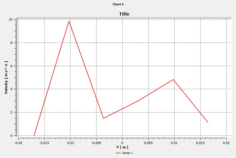
Line plot along the length of the pipe :

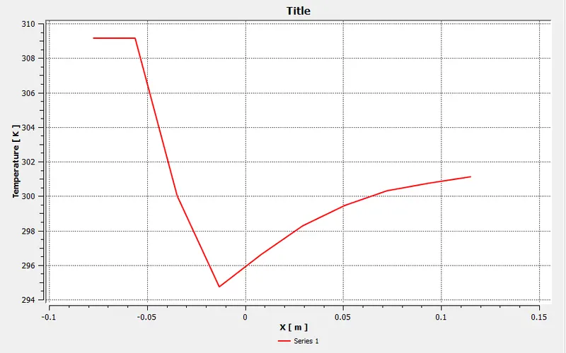
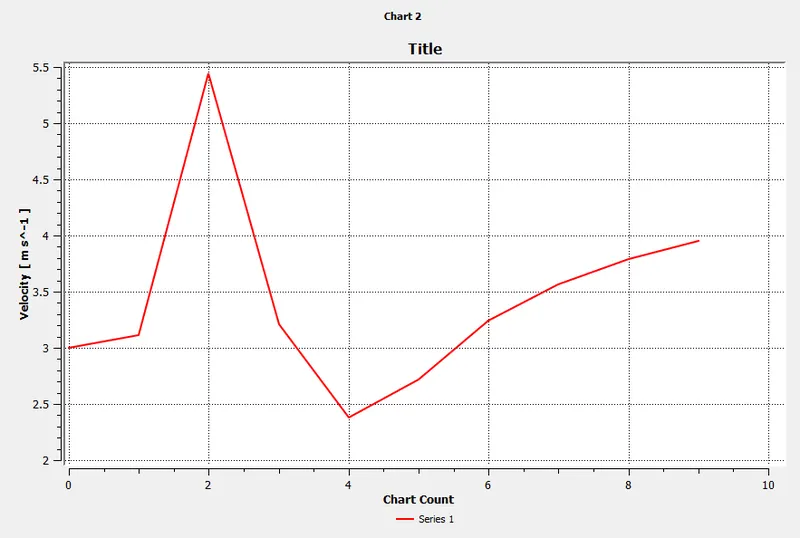
Line plot across the length of the pipe :

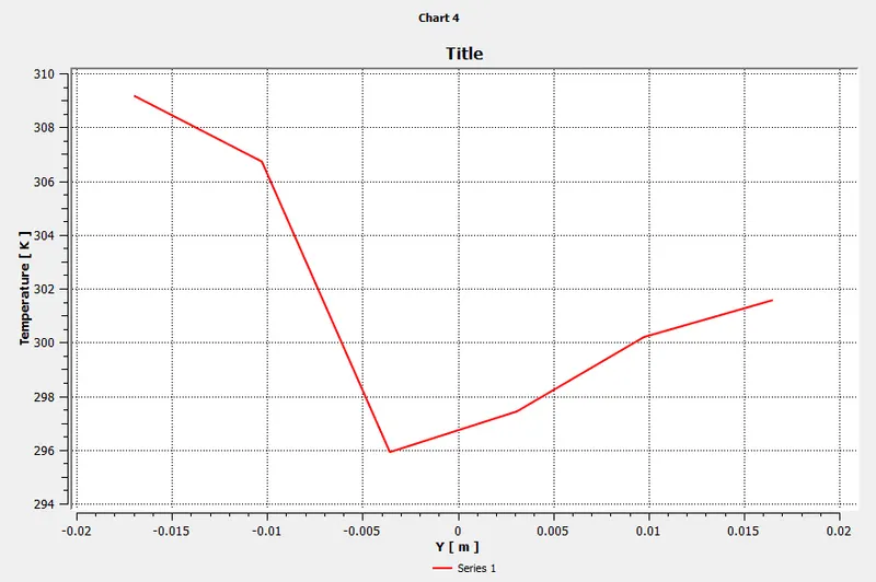
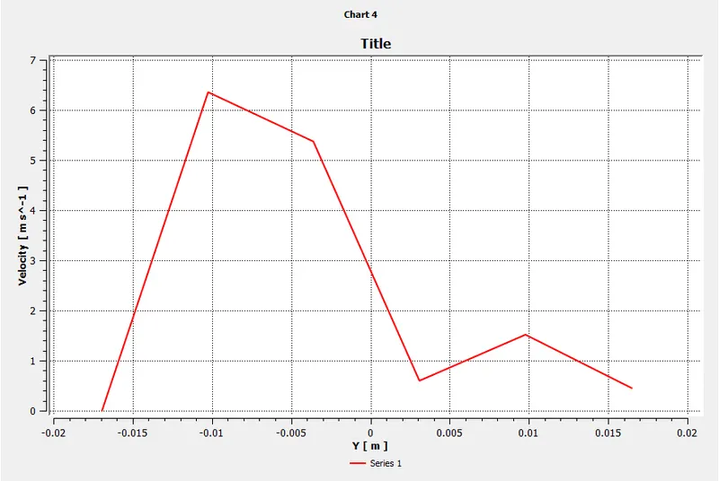
Subcase 2 :

For momentum ratio of 4 which hot air velocity = 3m/s and cold air velocity = 12m/s.

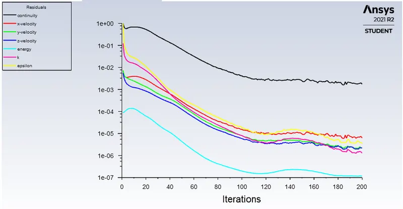
Residual plot :

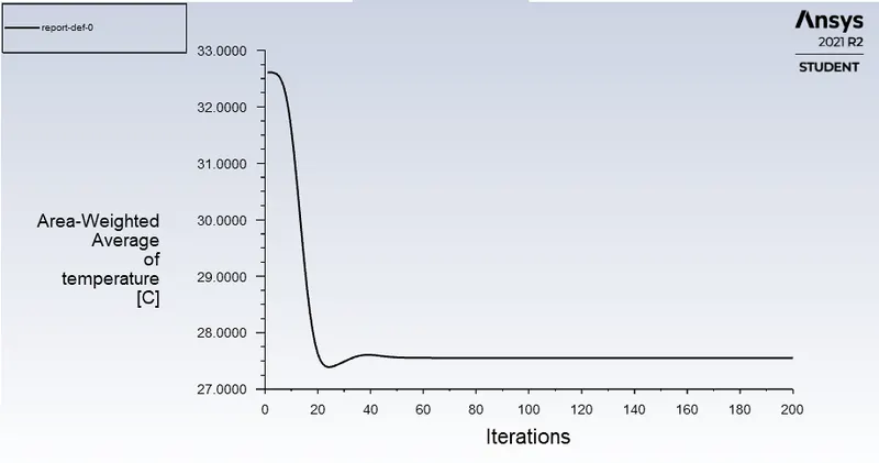
Average weighted area of temperature at the outlet :

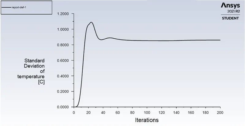
Standard deviation of temperature at outlet :

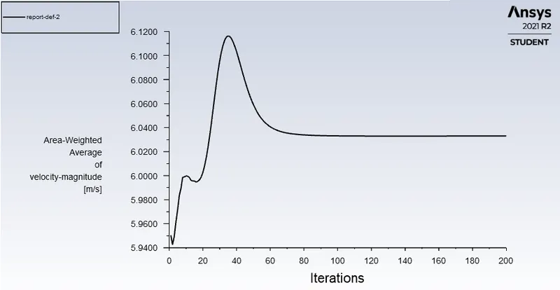
Average weighted area of velocity-magnitude at the outlet :

Contour plot :

1. For temperature distribution :

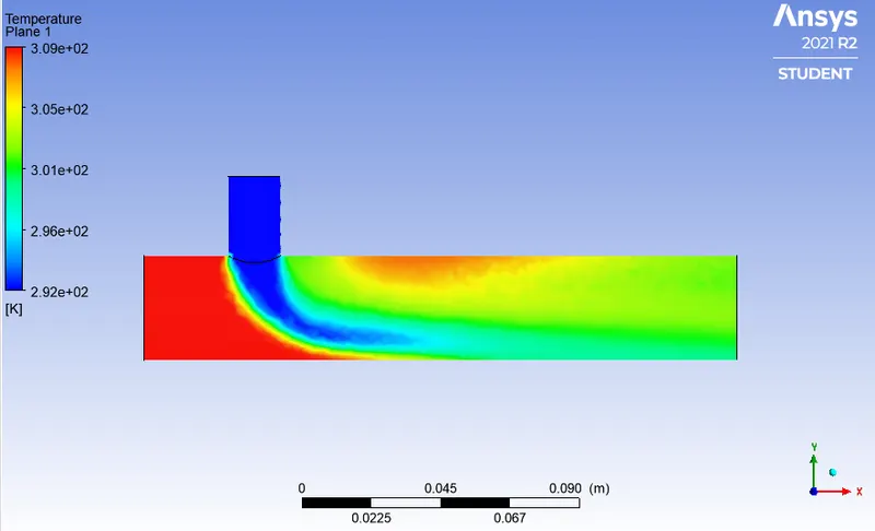
2. For velocity distribution :

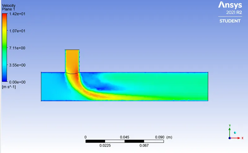
Line plot along the length of the pipe :

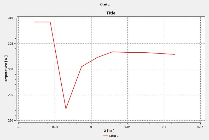
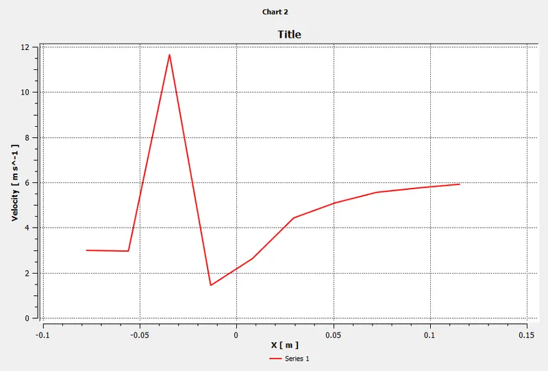
Line plot across the length of the pipe :

Validation of outlet temperature :

`T_(mixture) = ((m_(hot)*T_(hot) +m_(cold)*T_(cold))/(m_(hot)+m_(cold)))`

`m_(hot) = rho_(hot)*A*V_(hot)`

`m_(cold) = rho_(cold)*A*V_(cold)`

For subcase 1 :

Available data :

`bb(T_(hot))` = 36 degree celcius

`bb(T_(cold))` = 19 degree celcius

`A_(hot) = 901.3138mm^2`

`A_(cold) = 225.9823mm^2`

`bb(rho)` = 1.225kg/`m^3`

`bb(V_(cold))` = 6m/s

`bb(V_(hot))` = 3m/s

`T_(mixture) = 30.3` degree celcius.

For subcase 2 :

Available data :

`bb(T_(hot))` = 36 degree celcius

`bb(T_(cold))` = 19 degree celcius

`A_(hot) = 901.3138mm^2`

`A_(cold) = 225.9823mm^2`

`bb(rho)` = 1.225kg/`m^3`

`bb(V_(cold))` = 12m/s

`bb(V_(hot))` = 3m/s

`T_(mixture) = 27.48` degree celcius.

Cases1	Analytical value `T_(mixture)`	Numerical value `T_(mixture)`	Error(%)	Number of iterations required for convergence
Subcase 1	30.3 degree celcius	30.32 degree celcius	0.06	160
Subcase 2	27.48 degree celcius	27.57 degree celcius	0.32	180

Table(1)

From the above table we can say that the increase in velocity of a fluid is providing a better mixing of temperature at outlet.

Case 2 :

• Long mixing tee with a hot inlet velocity of 3m/s.
• Momentum ratio of 2, 4.

For momentum ratio of 2 :

Momentum ratio = velocity at cold inlet`(V_(cold))` / velocity at hot inlet`(V_(hot))`

2 = `(V_(cold))/3`

`bb(V_(cold))` = 6m/s

For momentum ratio of 4 :

Momentum ratio = velocity at cold inlet`(V_(cold))` / velocity at hot inlet`(V_(hot))`

4 = `(V_(cold))/3`

`bb(V_(cold))` = 12m/s.

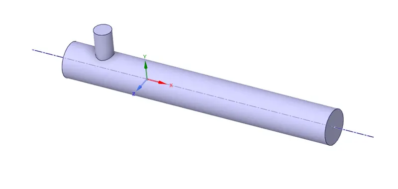
Geometry :

Import the step file of the geometry which is the short mixing tee in spaceclaim.

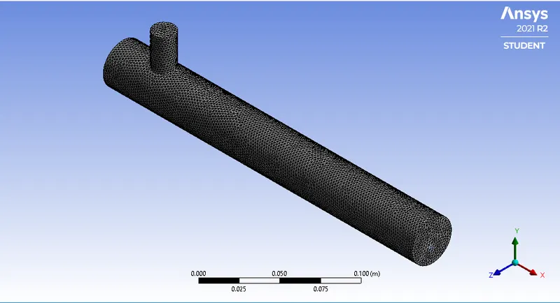
Mesh :

Body meshtype is slelected and we have done a mesh refinement for a element size of 0.004. The remain settings are default.

Element mesh quality :

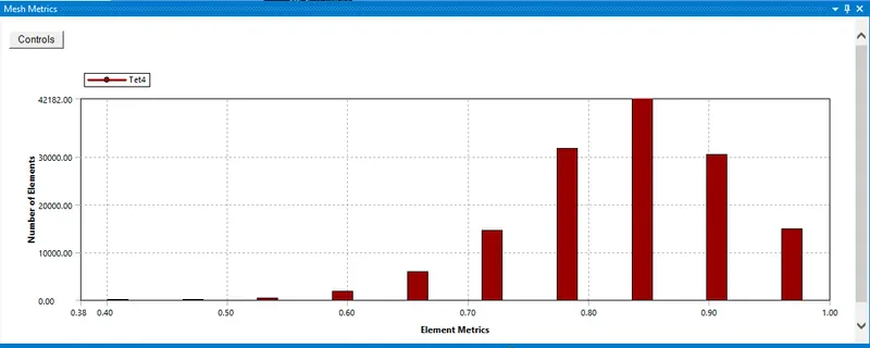
The above graph shows that the mesh quality of each element in that graph it is clear that the mesh quality ranges from minimum to maximum which is greater than 5% so it passes the test.

Number of elements and nodes :

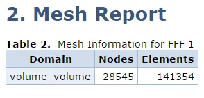
Then we need to name the geometry accordingly

1. Inlet x - Where as the hot air comes in.
2. Inlet y - Where as the cold air comes in.
3. Outlet x - Where the air exits.
4. Walls

Solution :

Short Tee for momentum ratio 2
Setup	k-epsilon
Solver type	pressure-based
Velocity formulation	Absolute
Time	Steady
Viscous model	Realizable k-epsilon with standard unction
Material	Air
cell zones volume-volume	Fluid type : Air
Boundaries	Inlet x (velocity inlet)
	velocity magnitude - 3m/s
	Temperature - 36 deg celcius
	Inlet y (velocity inlet)
	velocity magnitude - 12m/s
	Temperature - 19 deg celcius
	Outlet x (velocity outlet)
	Gauge pressure - 0pa
	Walls - stationary

Result :

Subcase 1 :

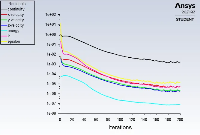
Residual plot :

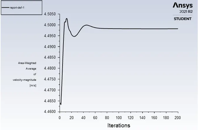
Average weighted area of velocity-magnitude at the outlet :

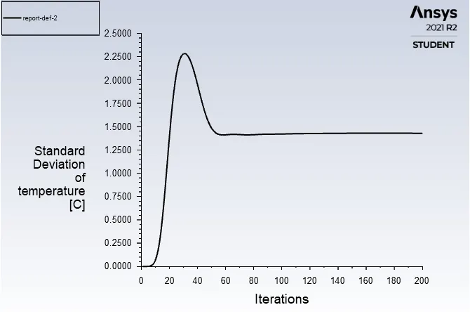
Standard deviation of temperature at outlet :

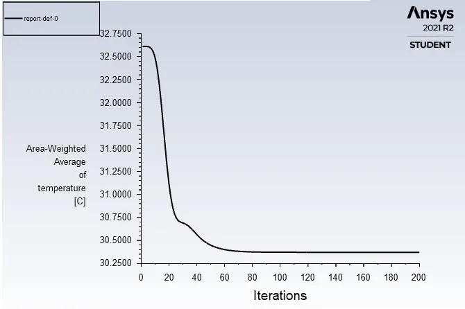
Average weighted area of temperature at the outlet :

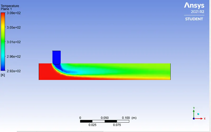
Contour plot :

1. For temperature distribution :

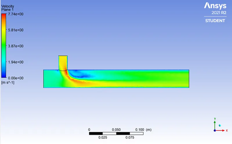
2. For velocity distribution :

Line plot along the length of the pipe :

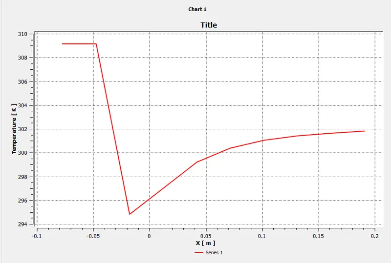
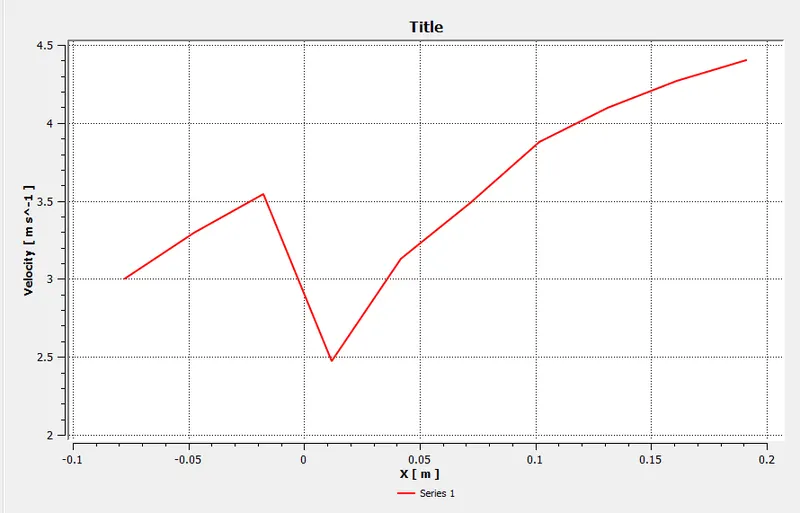
Line plot across the length of the pipe :

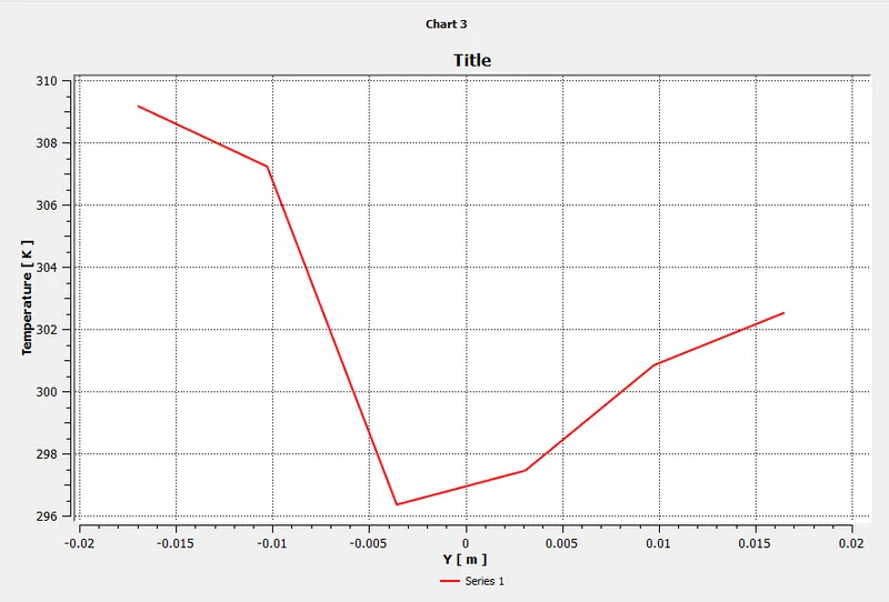
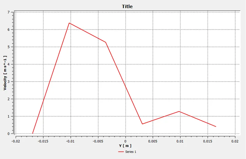
Subcase 2 :

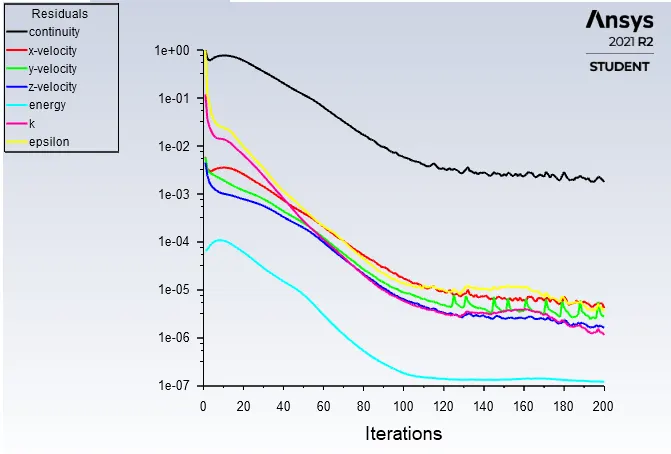
Residual plot :

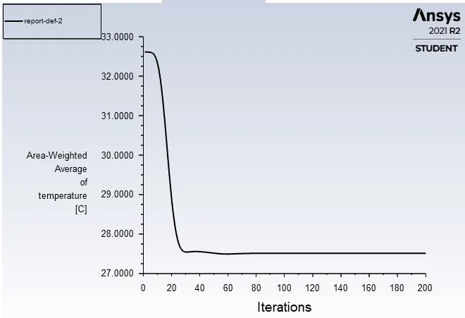
Average weighted area of temperature at the outlet :

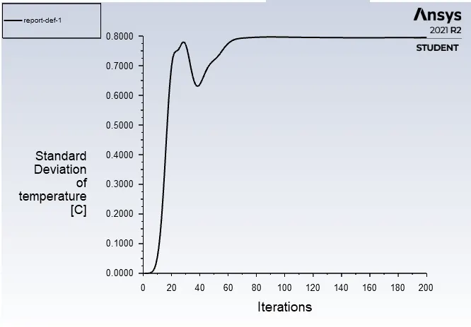
Standard deviation of temperature at outlet :

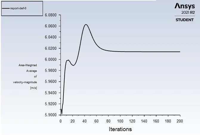
Average weighted area of velocity-magnitude at the outlet :

Contour plot :

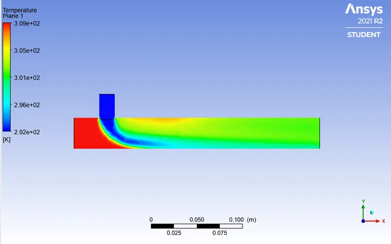
1. For temperature distribution :

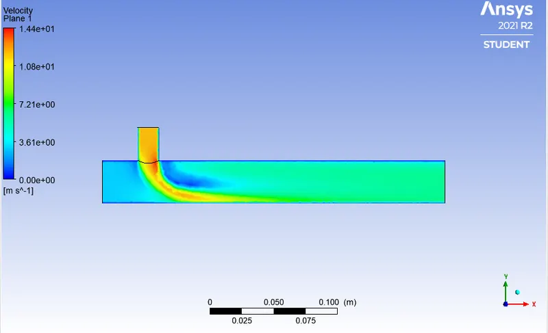
2. For velocity distribution :

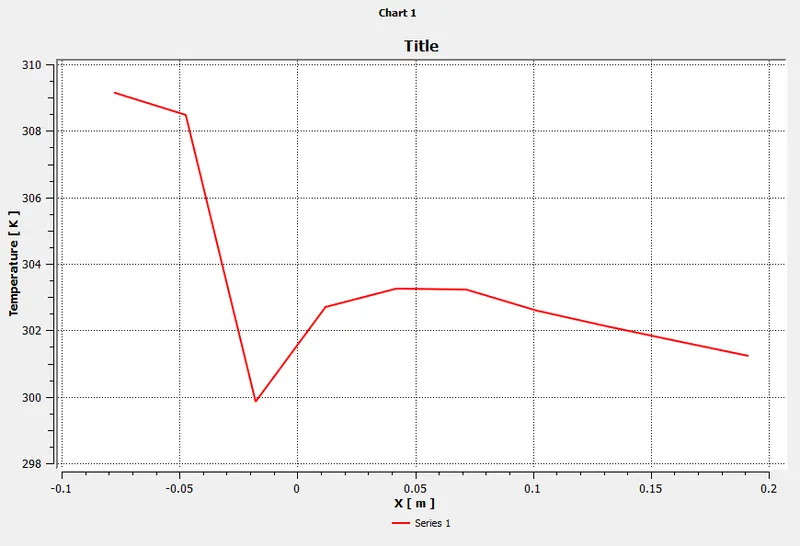
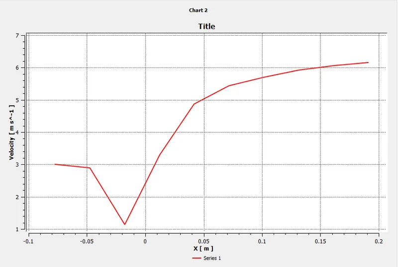
Line plot along the length of the pipe :

Line plot across the length of the pipe :

Validation of outlet temperature :

`T_(mixture) = ((m_(hot)*T_(hot) +m_(cold)*T_(cold))/(m_(hot)+m_(cold)))`

`m_(hot) = rho_(hot)*A*V_(hot)`

`m_(cold) = rho_(cold)*A*V_(cold)`

For subcase 1 :

Available data :

`bb(T_(hot))` = 36 degree celcius

`bb(T_(cold))` = 19 degree celcius

`A_(hot) = 901.3138mm^2`

`A_(cold) = 225.9823mm^2`

`bb(rho)` = 1.225kg/`m^3`

`bb(V_(cold))` = 6m/s

`bb(V_(hot))` = 3m/s

`T_(mixture) = 30.3` degree celcius.

For subcase 2 :

Available data :

`bb(T_(hot))` = 36 degree celcius

`bb(T_(cold))` = 19 degree celcius

`A_(hot) = 901.3138mm^2`

`A_(cold) = 225.9823mm^2`

`bb(rho)` = 1.225kg/`m^3`

`bb(V_(cold))` = 12m/s

`bb(V_(hot))` = 3m/s

`T_(mixture) = 27.48` degree celcius.

Cases1	Analytical value `T_(mixture)`	Numerical value `T_(mixture)`	Error(%)	Number of iterations took for convergence
Subcase 1	30.3 degree celcius	30.37 degree celcius	0.23	170
Subcase 2	27.48 degree celcius	27.50 degree celcius	0.20	190

Table(2)

After comparing Table(1) and Table(2) we can conclude that the increasing in length doesn't have any effect in the mixing of temperature at outlet and increasing the velocity provides a better mixng of temperature at outlet.

Conclusion :

• A fluid through a mixing tee to calculate the mixing effectiveness of the fluid at two different temperatures at the outlet of the mixing tee is successfully simulated and the results are discussed at the output.
• In the case of turbulence model k-epsilon provides a better results when compare to that of k-omega.
• Increasing the velocity of the cold inlet helps to increase the mixing efficiency.
• Increasing the length of the tee-joint doesn't made much impact in mixing.