Week 5.1 - Mid term project - Solving the steady and unsteady 2D heat conduction problem

Aim :

To write a matlab program to solve the steady and unsteady 2D heat conduction equation.

Objective :

• To solve steady and unsteady state 2D heat conduction equation by explicit an implicit method.
• While solving equations by implicit method iterations techniques such as Jacobi,Gauss-seidel & Successive over-relaxation are used.
• Then the solution meet the absolute error criteria of 1e-4 which is the acurracy of the solution.

Theory :

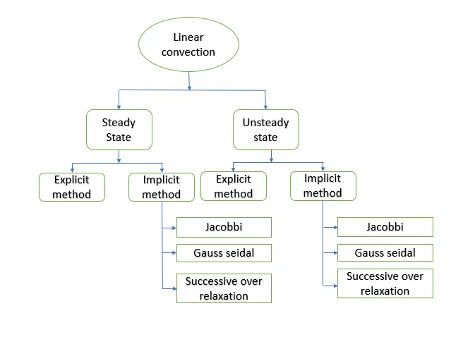
Numerical solution schemes are often referred to as being explicit or implicit. When a direct computation of the dependent variables can be made in terms of known quantities, the computation is said to be explicit. When the dependent variables are defined by coupled sets of equations, and either a matrix or iterative technique is needed to obtain the solution, the numerical method is said to be implicit.

Explicit method :

Explicit methods calculate the state of the system at a later time from the state of the system at the current time without the need to solve algebraic equations.

Implicit methods :

Implicit methods attempt to find a solution to the nonlinear system of equations iteratively by considering the current state of the system as well as its previous time state.

Iterative methods :

In computational mathematics, an iterative method is a mathematical procedure that uses an initial value to generate a sequence of improving approximate solutions for a class of problems, in which the n-th approximation is derived from the previous ones.

Types of iterative techniques :

1. Jacobbi method :

In jacobbi method we use the calculated value of the previous iteration in order to computed the current value.

2. Gauss seidal method :

In gauss seidal method we use the latest updated value in order to computed the value in the current state.

3. Sucessive over relaxation :

This type of iterative solver is used to improve the convergence rate by including a factor called relaxation factor.

Steady state and Unsteady heat conduction :

Heat transfer is the transfer of thermal energy from a body, at a high temperature, to another at a lower temperature. ... Under Steady state conditions the temperature within the system does not change with time.Conversely, under unsteady state conditions the temperature within the system does vary with time.

Boundary condition :

Steady state linear convection equation :

`(∂^2T)/(∂x^2)+(∂^2T)/(∂y^2) = 0`

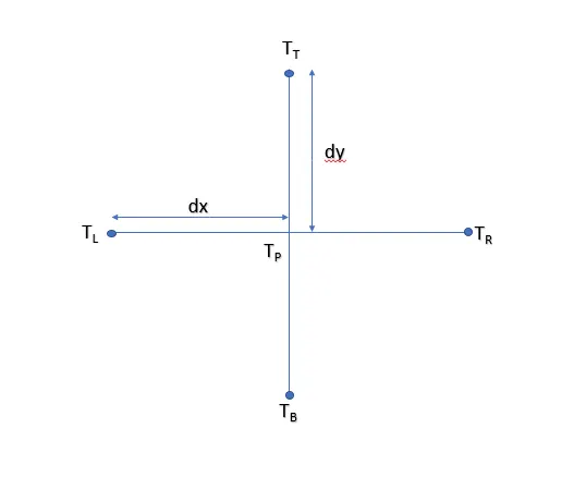
The above mentioned pde is of elliptic type so we use central differencing scheme

`(T(x-a)-2T(x)+T(x+a))/(dx^2) + (T(x-b)-2T(x)+T(x+b))/(dy^2)= 0`

`(2T_P)/(dx^2)+(2T_P)/(dy^2) =(T_L+T_R)/(dx^2) + (T_B+T_T)/(dy^2)`

`(2T_Pdy^2+2T_Pdx^2)/(dx^2dy^2) =(T_L+T_R)/(dx^2) + (T_B+T_T)/(dy^2)`

`T_P((2dy^2+2dx^2))/(dx^2dy^2) =(T_L+T_R)/(dx^2) + (T_B+T_T)/(dy^2)`

`T_P(k) =(T_L+T_R)/(dx^2) + (T_B+T_T)/(dy^2)`

`T_P =1/k((T_L+T_R)/(dx^2) + (T_B+T_T)/(dy^2))`

where as k = `(2dy^2+2dx^2)/(dx^2dy^2)`

Here explicit technique is same as that of the jacobi technique.

In case of implicit we have three different techniques which is jacobi, gauss seidal and successive over relaxation.

In Jacobi technique we use previously calculated iteration value to compute the current value.

In Gauss seidal technique we use the latest computed value to compute the current value.

In Successive over relaxation technique we use the following formula mentioned below

`T_p=(1-omega)T_(old)+omegaT_(gs)`

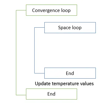
Pseudo code :

Unsteady state linear convection equation :

Explicit method :

`(∂^2T)/(∂t^2)-alpha((∂^2T)/(∂x^2)+(∂^2T)/(∂y^2)) = 0`

`(∂^2T)/(∂t^2)= alpha((∂^2T)/(∂x^2)+(∂^2T)/(∂y^2))`

In the above mentioned pde time derivative is solved using forward difference scheme and space derivative is of elliptic type so we use central differencing scheme to solve that equation.

`(T(x+a)-T(x))/(dt^2)=alpha((T(x-a)-2T(x)+T(x+a))/(dx^2) + (T(x-b)-2T(x)+T(x+b))/(dy^2))`

`T_(p2)=T_(old)+(alpha.dt^2)((T_L-2T_P+T_R))/(dx^2) + (alpha.dt^2)((T_B-2T_P+T_T))/(dy^2)`

`T_(p2)=T_(old)+K_1(T_L-2T_P+T_R) + K_2(T_B-2T_P+T_T)`

Where as `K_1 = (alpha.dt^2)/(dx^2)` and `K_2 = (alpha.dt^2)/(dy^2)`

Implicit method :

`(∂^2T)/(∂t^2)-alpha((∂^2T)/(∂x^2)+(∂^2T)/(∂y^2)) = 0`

`(∂^2T)/(∂t^2)= alpha((∂^2T)/(∂x^2)+(∂^2T)/(∂y^2))`

In the above mentioned pde time derivative is solved using forward difference scheme and space derivative is of elliptic type so we use central differencing scheme to solve that equation.

`(T(x+a)-T(x))/(dt^2)=alpha((T(x-a)-2T(x)+T(x+a))/(dx^2) + (T(x-b)-2T(x)+T(x+b))/(dy^2))`

`T_p+alpha((2T_P)/(dx^2))dt^2+alpha((2T_P)/(dy^2))dt^2 =T_(previous)+alpha.dt^2((T_L+T_R)/(dx^2) + (T_B+T_T)/(dy^2))`

`T_P(1+((2alpha)/(dx^2))dt^2+((2alpha)/(dy^2))dt^2) =T_(previous)+alpha.dt^2((T_L+T_R))/(dx^2) + alpha.dt^2((T_B+T_T))/(dy^2)`

`T_P(1+2K_1+2K_2) =T_(previous)+K_1(T_L+T_R) + K_2(T_B+T_T)`

`T_P = 1/(1+2K_1+2K_2)(T_(previous)+K_1(T_L+T_R) + K_2(T_B+T_T))`

where as `K1 =((dt^2alpha)/(dx^2))` and `K2 =((dt^2alpha)/(dy^2))`

In case of implicit we have three different techniques which is jacobi, gauss seidal and gauss elimiation.

In Jacobi technique we use previously calculated iteration value to compute the current value.

In Gauss seidal technique we use the latest computed value to compute the current value.

In Successive over relaxation technique we use the following formula mentioned below

`T_p=(1-omega)T_(old)+omegaT_(gs)`

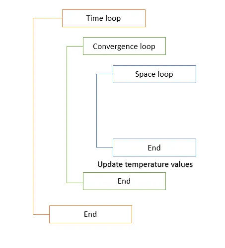
Pseudo code :

Data's we have :

Domain length towards x-axis = 1m.

Domain length towards y-axis = 1m.

Top Boundary temperature = 600 K.

Bottom Boundary temperature = 900 K.

Left Boundary temperature = 400 K.

Right Boundary temperature = 800 K.

Thermal diffusivity = 1.1

Relaxation factor = 1.1

Assume number of node points = 10 (Both x and y axis)

Timestep = 1e-3.

Steady state implicit method :

Program :

% Code to solve steady state 2-D heat conduction problem
% Steady state solver
% Iterative methods - Jacobbi, Gauss seidal, Successive over relaxation.

clear all 
close all
clc

% Inputs
nx = 10;
ny = 10;
Tx = linspace(0,1,nx)
Ty = linspace(0,1,ny)


% Definng grid size
dx = 1/(nx-1);
dy = 1/(ny-1);

%Defining boundary condition
T = 300*ones(nx,ny)

% Defining initial condition
% Temperature at the top of the boundary(Tt) = 600
% Temperature at the top of the boundary(Tb) = 900
% Temperature at the top of the boundary(Tl) = 400
% Temperature at the top of the boundary(Tr) = 800

T(1,:) = 600
T(nx,:) = 900
T(:,1) = 400
T(:,ny) = 800

Tt = 600;
Tb = 900;
Tl = 400;
Tr = 800;

% Defining corner temperatures
T(1,1) = (Tt+Tl)/2;
T(1,ny) = (Tt+Tr)/2;
T(nx,1) = (Tb+Tl)/2;
T(nx,ny) = (Tb+Tr)/2;

% creating a copy of T
Told = T;
error = 9e9;
tol = 1e-4;
iterative_solver = 1;

% jacobi method
% steady state
% d^2T/dx^2+d^2T/dy^2 = 0

 k = (2*dy^2+2*dx^2)/(dx^2*dy^2)
 w = 1.1

if iterative_solver == 1
    jacobi_iter = 1;
    tic
    while(error > tol)
        for i = 2:nx-1
            for j = 2:ny-1
             T(i,j) = (1/k)*((Told(i-1,j)+Told(i+1,j))/(dx^2)+(Told(i,j-1)+Told(i,j+1))/(dy^2));
            end
        end      
        error = max(max(abs(Told-T)));
        Told = T;
        jacobi_iter=jacobi_iter+1;
        contourf(Tx,Ty,T,'ShowText','on')
        colorbar
        colormap(jet)
        set(gca, 'ydir', 'reverse')
        xlabel('x-axis')
        ylabel('velocity')
        title_text = sprintf('Total number of iteration = %d for implicit method(jacobi)',jacobi_iter);
        title(title_text)
        pause(0.03)
        
    end
    toc
    simulation_time_jacobi = toc
end



% Gauss seidal method
tic
if iterative_solver == 2
    Gauss_seidal_iter = 1;
    while(error > tol)
        for i = 2:nx-1
            for j = 2:ny-1
                 T(i,j) = (1/k)*((T(i-1,j)+T(i+1,j))/(dx^2)+(T(i,j-1)+T(i,j+1))/(dy^2));
            end
        end      
        error = max(max(abs(Told-T)));
        Told = T;
        Gauss_seidal_iter = Gauss_seidal_iter+1;
        contourf(Tx,Ty,T,'ShowText','on')
        colorbar
        colormap(jet)
        set(gca, 'ydir', 'reverse')
        xlabel('x-axis')
        ylabel('velocity')
        title_text = sprintf('Total number of iteration = %d for implicit method(Gauss seidal)',Gauss_seidal_iter);
        title(title_text)
        pause(0.03)
        
    end
    toc
    simulation_time_gs = toc

end

% Successive over relaxation method
tic
if iterative_solver == 3
    SOR_iter = 1;
    while(error > tol)
        for i = 2:nx-1
            for j = 2:ny-1
                 T(i,j) = (1-w)*Told(i,j) + w*((1/k)*((T(i-1,j)+T(i+1,j))/(dx^2)+(T(i,j-1)+T(i,j+1))/(dy^2)));
            end
        end      
        error = max(max(abs(Told-T)));
        Told = T;
        SOR_iter = SOR_iter+1;
        contourf(Tx,Ty,T,'ShowText','on')
        colorbar
        colormap(jet)
        set(gca, 'ydir', 'reverse')
        xlabel('x-axis')
        ylabel('velocity')
        title_text = sprintf('Total number of iterations = %d for implicit method(SOR)',SOR_iter);
        title(title_text)
        pause(0.03)
        
    end
    toc
    simulation_time_SOR = toc
end

Output :

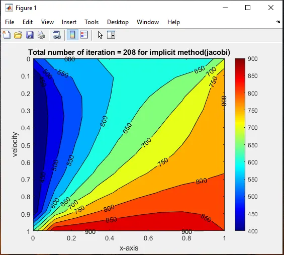
figure(1)

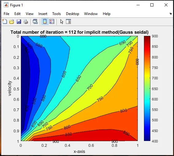
figure(2)

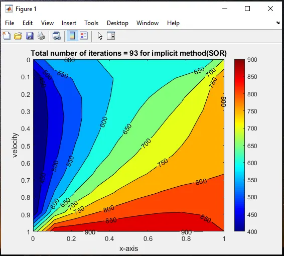
figure(3)

Unsteady state explicit method :

Program :

% Code to solve unsteady/Transient state 2-D heat conduction problem
% Unsteady state solver
% Explicit method.
clear all 
close all
clc

% Inputs
nx = 10;
ny = 10;
Tx = linspace(0,1,nx)
Ty = linspace(0,1,ny)


% Defining grid size
dx = 1/(nx-1);
dy = 1/(ny-1);

% Defining boundary condition
T = 300*ones(nx,ny)

% Defining initial condition
% Temperature at the top of the boundary(Tt) = 600
% Temperature at the top of the boundary(Tb) = 900
% Temperature at the top of the boundary(Tl) = 400
% Temperature at the top of the boundary(Tr) = 800

T(1,:) = 600
T(nx,:) = 900
T(:,1) = 400
T(:,ny) = 800

Tt = 600;
Tb = 900;
Tl = 400;
Tr = 800;

% Defining corner temperatures
T(1,1) = (Tt+Tl)/2;
T(1,ny) = (Tt+Tr)/2;
T(nx,1) = (Tb+Tl)/2;
T(nx,ny) = (Tb+Tr)/2;

% creating a copy of T
Told = T;
Tprev = T;
error = 9e9;
tol = 1e-4;
alpha = 1.1;
dt = 1e-3;

% jacobi method
% Unsteady state

 k1 = (alpha*dt)/(dx^2);
 k2 = (alpha*dt)/(dy^2);

 Explicit_solver = 1;
 tic
 for k=1:1400
         for i = 2:nx-1
             for j = 2:ny-1
                 term1 = (Told(i-1,j)-2*Told(i,j)+Told(i+1,j));
                 term2 = (Told(i,j-1)-2*Told(i,j)+Told(i,j+1));
                 T(i,j) = Told(i,j)+(k1*term1)+(k2*term2);
             end
         end      
         Told = T;
         Explicit_solver=Explicit_solver+1;
         contourf(Tx,Ty,T,'ShowText','on')
         colorbar
         colormap(jet)
         xlabel('x-axis')
         ylabel('velocity')
         title_text = sprintf('Total number of iterations for Explicit method = %d',Explicit_solver);
         title(title_text)
         set(gca, 'ydir', 'reverse')
         pause(0.03)
 end
simulation_time = toc

Output :

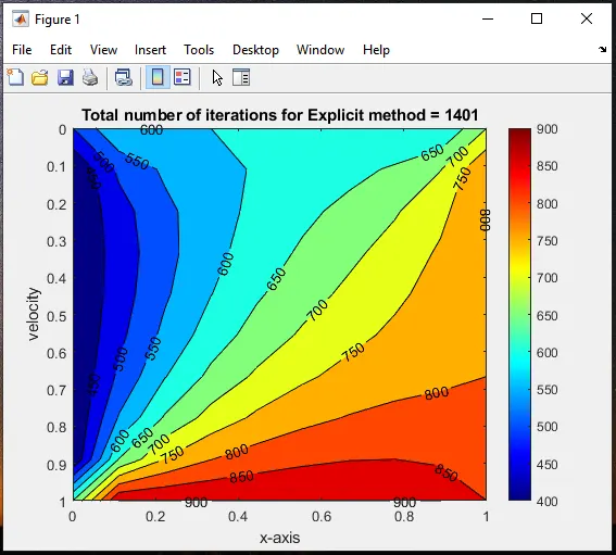
figure(4)

Program :

% Code to solve unsteady/Transient state 2-D heat conduction problem
% Unsteady state solver
% Iterative methods - Jacobbi, Gauss seidal, Successive over relaxation.

clear all 
close all
clc

% Inputs
nx = 10;
ny = 10;
Tx = linspace(0,1,nx)
Ty = linspace(0,1,ny)


% Definng grid size
dx = 1/(nx-1);
dy = 1/(ny-1);

%Defining boundary condition
T = 300*ones(nx,ny)

% Defining initial condition
% Temperature at the top of the boundary(Tt) = 600
% Temperature at the top of the boundary(Tb) = 900
% Temperature at the top of the boundary(Tl) = 400
% Temperature at the top of the boundary(Tr) = 800

T(1,:) = 600
T(nx,:) = 900
T(:,1) = 400
T(:,ny) = 800

Tt = 600;
Tb = 900;
Tl = 400;
Tr = 800;

% Defining corner temperatures
T(1,1) = (Tt+Tl)/2;
T(1,ny) = (Tt+Tr)/2;
T(nx,1) = (Tb+Tl)/2;
T(nx,ny) = (Tb+Tr)/2;

% creating a copy of T
Told = T;
Tprev = T;

%Inputs
error = 9e9;
tol = 1e-4;
alpha = 1.1;
dt = 1e-3;
iterative_solver = 1;
k1 = (alpha*dt)/(dx^2);
k2 = (alpha*dt)/(dy^2)
w = 1.1;


% jacobi method
% unsteady state
 
if iterative_solver == 1
    jacobi_iter = 1;
    tic
    for k=1:1400
        error = 9e9;
        while(error > tol)
            for i = 2:nx-1
                for j = 2:ny-1
                    term1 = 1/(1+2*k1+2*k2);
                    term2 = k1*term1;
                    term3 = k2*term1;
                    H = (Told(i-1,j)+Told(i+1,j));
                    V = (Told(i,j-1)+Told(i,j+1));
                    T(i,j) =(term1*Tprev(i,j)+term2*H+term3*V);
                end
            end      
            error = max(max(abs(Told-T)));
            Told = T;
            jacobi_iter=jacobi_iter+1;
            contourf(Tx,Ty,T,'ShowText','on')
            colorbar
            colormap(jet)
            set(gca, 'ydir', 'reverse')
            xlabel('x-axis')
            ylabel('velocity')
            title_text = sprintf('Total number of iteration = %d for implicit method(jacobi)',jacobi_iter);
            title(title_text)
            pause(0.03)
        end
          Tprev = Told;
    end
    toc
    simulation_time_jacobi = toc 
end



% Gauss seidal method
if iterative_solver == 2
    gauss_seidal_iter = 1;
    tic
    for k=1:1400
        error = 9e9;
        while(error > tol)
            for i = 2:nx-1
                for j = 2:ny-1
                    term1 = 1/(1+2*k1+2*k2);
                    term2 = k1*term1;
                    term3 = k2*term1;
                    H = (T(i-1,j)+T(i+1,j));
                    V = (T(i,j-1)+T(i,j+1));
                    T(i,j) =(term1*Tprev(i,j)+term2*H+term3*V);
                end
            end      
            error = max(max(abs(Told-T)));
            Told = T;
            gauss_seidal_iter=gauss_seidal_iter+1;
            contourf(Tx,Ty,T,'ShowText','on')
            colorbar
            colormap(jet)
            set(gca, 'ydir', 'reverse')
            xlabel('x-axis')
            ylabel('velocity')
            title_text = sprintf('Total number of iteration = %d for implicit method(Gauss seidal)',gauss_seidal_iter);
            title(title_text)
            pause(0.03)
        end
        Tprev = Told;
    end
    toc
    simulation_time_gs = toc    
end

% Successive over relaxation method
if iterative_solver == 3
    SOR_iter = 1;
    tic
    for k=1:1400
        error = 9e9;
        while(error > tol)
            for i = 2:nx-1
                for j = 2:ny-1
                    term1 = 1/(1+2*k1+2*k2);
                    term2 = k1*term1;
                    term3 = k2*term1;
                    H = (T(i-1,j)+T(i+1,j));
                    V = (T(i,j-1)+T(i,j+1));
                    T(i,j)=(1-w)*Told(i,j)+w*(term1*Tprev(i,j)+term2*H+term3*V);
                end
            end      
            error = max(max(abs(Told-T)));
            Told = T;
            SOR_iter=SOR_iter+1;
            contourf(Tx,Ty,T,'ShowText','on')
            colorbar
            colormap(jet)
            set(gca, 'ydir', 'reverse')
            xlabel('x-axis')
            ylabel('velocity')
            title_text = sprintf('Total number of iteration = %d for implicit method(SOR)',SOR_iter);
            title(title_text)
            pause(0.03)
        end
        Tprev = Told;
    end
    toc
    simulation_time_SOR = toc
end

Output :

Unsteady state implicit method :

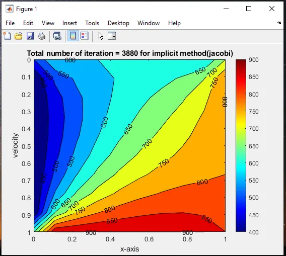
figure(5)

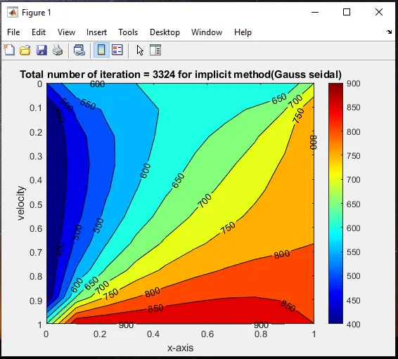
figure(6)

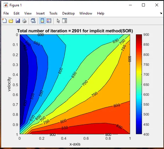
figure(7)

Implicit method (Unsteady/Transient state)
Iterative techniques	No. of iterations
Jacobi	3880
Gauss seidal	3324
SOR	2901

Table(1)

Implicit method (Steady state)
Iterative techniques	No. of iterations
Jacobi	208
Gauss seidal	112
SOR	93

Table(2)

Total number of iterations in unsteady state explicit mehod = 1401

Discussion of output :

• From the analysis it is clear that the steady state condition requires comparetively less number of iteration and less computational time when compare to that of transient state system in order to converge a result.
• In case of implicit method in both steady and unsteady state jocobi technique requires more number of iteration and the followed by gauss seidal and then finally succesive over relaxation technique.
• Jacobi>Gauss seidal>Successive over relaxation.
• The successsive over relaxation technique has minimum iteration this is because of the relaxation factor here we used `omega = 1.1` which is over relaxed which helps to converge a result in a faster rate.
• While comparing the solution of unsteady state explicit and implicit method, Explicit method consumes very less number of iteration to converge a result and it requires less computational time than implicit. Eventhough it consumes less number of iterations both the method has certain advantages when time accurate solution is needed explicit method is preferred.
• when steady state answer are desired implicit methods are preferred.

Conclusion :

• A matlab program for steady and unsteady state 2D heat conduction equation is solved using both explicit and implicit method is successfully compiled and the results are discussed in the output.