Project 2 - Rankine cycle Simulator

Aim :

To create a Rankine cycle simulator using matlab and to plot a T-S and H-S diagram.

Objective :

• To create a rankine cyle simulator.
• To calculate state values of a rankine cycle based on user inputs.
• To plot the corresponding T-s and h-s plots for the given set of inputs.
• To calculate net work output and Back work ratio.

Theory :

Rankine cycle :

The Rankine cycle is founded by William John Macquorn Rankine a Scottish engineer and physicist in 1859. He was a founding contributor to the science of thermodynamics. Rankine developed a complete theory of the steam engine and indeed of all heat engines.

Rankine cycle is a power producing cycle and widely used in steam based power plants. The main principle of Rankine cycle is to produce a high pressure and temperature steam which strikes the turbine blades and rotates the turbine with high speed and the it is coupled with generator which converts the mechanical energy into electrical energy.

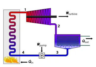
fig(1)

The heat sources used in these power plants are usually nuclear fission or the combustion of fossil fuels such as coal, natural gas, and oil. The Rankine Cycle’s major components include a rotating steam turbine, pump, stationary condenser and a boiler. The working fluid in a rankine cycle follows a closed loop and it is reused constantly.

fig(2)

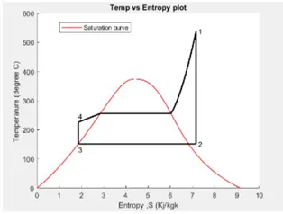
There are four processes in the Rankine cycle. These states are identified by numbers in the above T-s diagram.

• Process 1-2: It is an isentropic expansion process where the dry saturated vapour expands through a turbine, generating power. This decreases the temperature and pressure of the vapour, and some condensation may occur.
• Process 2-3: The wet vapour then enters a condensor where it is condensed at a constant pressure to become a saturated liquid.
• Process 3-4: The working fluid is pumped from low to high pressure. As the fluid is a liquid at this stage, the pump requires little input energy.
• Process 4-1: The high pressure liquid enters a boiler where it is heated at constant pressure by an external heat source to become a dry saturated vapour.

Efficiency of Rankine Cycles :

• Efficiency of rankine cycle is comparatively less when compare to that of a carnot cycle because in carnot cycle heat and addition and rejection takes place isothermally which is practically impossible and it is a reversible cycle no heat loss takes place in this cycle.
• In rankine cycle heat addidtion and rejection takes place at constant pressure and it is an irreversible process.

The efficiency of the Rankine cycle is improved :

Superheating and reheating :

• The irreversibility of any process is reduced if it is performed as close as possible to the temperatures of the high temperature and low temperature reservoirs. This is achieved by operating the condenser at subatmospheric pressure. The temperature in the boiler is limited by the saturation pressure. Further increase in temperature is possible by superheating the saturated vapor.

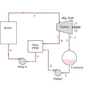
Feed water preheating :

• The cold liquid leaving the feed pump is mixed with the saturated liquid in the boiler and/or re-heated to the boiling temperature. The resulting irreversibility reduces the efficiency of the boiler. According to the Carnot process, the highest efficiency is reached if heat transfer occurs isothermally. To preheat the feed liquid to its saturation temperature, bleed vapor from various positions of the turbine is passed through external heat exchangers (regenerators). Ideally, the temperature of the bleed steam should be as close as possible to the temperature of the feed liquid.

Combined cycles :

• The high combustion temperature of the fuel is better utilized if a gas turbine or Brayton engine is used as "topping cycle" in conjunction with a Rankine cycle. In this case, the hot gas leaving the turbine is used to provide the energy input to the boiler. In co-generation systems, the energy rejected by the Rankine cycle is used for space heating, process steam or other low temperature applications.

Based on the fig(2) the formula has been derived to calculate the followings

Turbine Work (KJ/Kg)

Wt = h1 – h2

Pump Work (KJ/Kg)

Wp = v3 x (p4 – p3) x 100

Net Work (KJ/Kg)

Wnet = Wt + Wp

Specific steam consumption (Kg/Kwh)

SSC = 3600/Wnet

Heat supplied (KJ/Kg)

Qin = h1 - h4

Heat rejected (KJ/Kg)

Qout = h2 - h3

Thermal Efficiency (%)

T_eff = (Wnet/Qin) x 100

Back work ratio

BW = Wp/Wt

PROGRAM :

clear all
close all
clc

% printing Introduction
fprintf('Rakine cycle simulator\n');
fprintf('1-2 is Isentropic expansion in turbine \n');
fprintf('2-3 Constant pressure heat rejection by the condensor\n');
fprintf('3-4 is Isentropic compression in pump\n');
fprintf('2-3 Constant pressure heat addition by the boiler\n');

% User Inputs
p1 = input('\n Enter the value pressure at the turbine inlet in bar\n');
t1 = input('Enter the temperature at the turbine inlet in degree celcius\n');
p2 = input('Enter the value pressure at the turbine outlet in bar\n');


% State point 1
h1  = XSteam('h_pT',p1,t1);
s1  = XSteam('s_pT',p1,t1);

% State point 2
s2  = s1;
sf2 = XSteam('sL_p',p2);
sg2 = XSteam('sV_p',p2);
x   = (s2-sf2)/(sg2-sf2);
hf2 = XSteam('hL_p',p2);
hg2 = XSteam('hV_p',p2);
h2  = hf2+x*(hg2-hf2);
ts2  = XSteam('Tsat_p',p2);
t2 = XSteam('T_ph',p2,h2);
if x>=1
    t2=ts2;
end

% State point 3
h3 = hf2;
s3 = sf2;
p3 = p2;
t3 = t2;

% State point 4
p4 = p1;
s4 = s3;
h4  = XSteam('h_ps',p4,s4);
t4  = XSteam('T_ps',p4,s4);

% workdone by turbine

Wt = h1 -h2;

% workdone by pump
v3 = XSteam('vL_p',p3);
Wp = v3*(p4-p3)*100;

% net work done
Wnet = Wt - Wp;

% Heat suplied into the system
Qin = h1 - h4;

% Heat rejected from the system
Qout = h2 - h3;

% Thermal efficiency
T_eff = (Wnet/Qin)*100;

% Specific steam consumption
SSC = (3600/Wnet);

% Back work ratio
BW = (Wp/Wt);

% Saturation liguid and vapour point calculation

hf1 = XSteam('hL_p',p1);
hg1 = XSteam('hV_p',p1);
ts1  = XSteam('Tsat_p',p1);
sf1 = XSteam('sL_p',p1);
sg1 = XSteam('sV_p',p1);
t5 = ts1;

% printing results
fprintf('\nResults\n');
fprintf('\nAt State point1:\np1 = %4.2f Bar\nt1 = %4.2f degree celcius\nh1 = %4.2f KJ/Kg\ns1 = %4.2f KJ/kgK\n',p1,t1,h1,s1)
fprintf('\nAt State point2:\np2 = %4.2f Bar\nt2 = %4.2f degree celcius\nh2 = %4.2f KJ/Kg\ns2 = %4.2f KJ/kgK\n',p2,t2,h2,s2)
fprintf('\nAt State point3:\np3 = %4.2f Bar\nt3 = %4.2f degree celcius\nh3 = %4.2f KJ/Kg\ns3 = %4.2f KJ/kgK\n',p3,t3,h3,s3)
fprintf('\nAt State point4:\np4 = %4.2f Bar\nt4 = %4.2f degree celcius\nh4 = %4.2f KJ/Kg\ns4 = %4.2f KJ/kgK\n',p4,t4,h4,s4)
fprintf('\nWt = %4.2f KJ/Kg\nWp = %4.2f KJ/Kg\nWnet = %4.2f KJ/Kg\nThermal Efficiency = %4.2f Percent\nSSC = %4.2fKg/Kwh\nBack work ratio = %4.4f\n',Wt,Wp,Wnet,T_eff,SSC,BW)


% Plotting Saturation curve and T-s diagram

figure(1)
hold on

t = linspace(1,800,1000);

% plotting saturation curve

for i = 1:length(t)
plot(XSteam('sL_T',t(i)),t(i),'.','color','r');
plot(XSteam('sV_T',t(i)),t(i),'.','color','r');

end

% plotting T-S curve

plot([s1 s2],[t1 t2],'color','b','linewidth',1);
plot([s2 s3],[t2 t3],'color','b','linewidth',1);
plot([s3 s4],[t3 t4],'color','b','linewidth',1);
plot([s4 sf1],[t4 t5],'color','b','linewidth',1);
plot([sf1 sg1],[t5 ts1],'color','b','linewidth',1);
plot([sg1 s1],[ts1 t1],'color','b','linewidth',1);

text(s1+0.2,t1,'1');
text(s2+0.2,t2,'2');
text(s3+0.1,t3-8,'3');
text(s4-0.2,t4+8,'4');
text(sf1-0.4,t5+5,'5');
text(sg1+0.1,ts1,'6');

xlabel('Entropy in KJ/KgK')
ylabel('Temperature in K')
title('T-S diagram')
legend('saturation curve')

% Plotting saturation curve and h-s diagram

figure(2)
hold on

% plotting saturation curve 

for i = 1:length(t)
plot(XSteam('sL_T',t(i)),XSteam('hL_T',t(i)),'.','color','r','linewidth',1);
plot(XSteam('sV_T',t(i)),XSteam('hV_T',t(i)),'.','color','r','linewidth',1);
end

% plotting h-S curve
plot([s1 s2],[h1 h2],'color','b','linewidth',1);
plot([s2 s3],[h2 h3],'color','b','linewidth',1);
plot([s3 s4],[h3 h4],'color','b','linewidth',1);
plot([s4 s1],[h4 h1],'color','b','linewidth',1);


text(s1+0.2,h1,'1');
text(s2+0.2,h2,'2');
text(s3+0.2,h3-9,'3');
text(s4-0.3,h4+12,'4');

xlabel('Entropy in KJ/KgK')
ylabel('Enthalpy in KJ/K')
title('h-S diagram')
legend('saturation curve')

PROGRAM EXPLANATION :

• Firstly explain the processes using fprintf command.
• Get the inputs from the user such as p1,t1 and p2 using input command.
• Then calculate the state values such as Entropy(s), Enthalpy(h), Pressure(p), Temperature(t) at each state using XSteam data file.
• Then calculate turbine work(Wt), pump work(Wp), specific steam consumption(SSC), Heat supplied(Qin), Heat rejected(Qut), Thermal efficiency(T_eff) and Back work ratio(BW) using the state parameters.
• Then display all the above calculated values using fprintf command.
• Then get the temperature value in between 1 to 800 for 1000 intervals using linspace command.
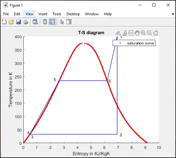
• Then plot for T-s and h-s diagram. For h-s and T-s plot we need to draw a saturation curve for that we used for loop give the size of a for loop, in our code for loop size is equal to the length of the temperature, for each temperature value saturated values of entropy and enthalpy has been found and ploted.
• Then plot the results of Temperature and Entropy in each state using plot command and name that figure has figure(1) using figure command.
• Then number the states using text command then give appropriate title using title command.
• Then name xaxis and yaxis using xlabel and ylabel command.
• Then plot the results of Enthalpy and Entropy in each state using plot command and name that figure has figure(2) using figure command.
• Then number the states using text command then give appropriate title using title command.
• Then name xaxis and yaxis using xlabel and ylabel command.
• Finally legend command is used to define the type of curve used.

Results :

T-S plot :

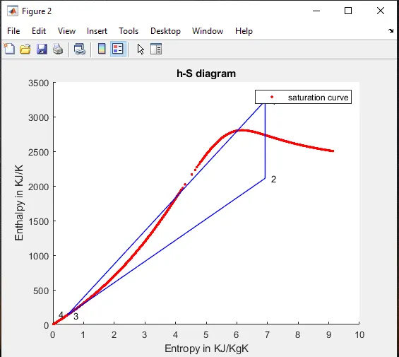
h-S plot :

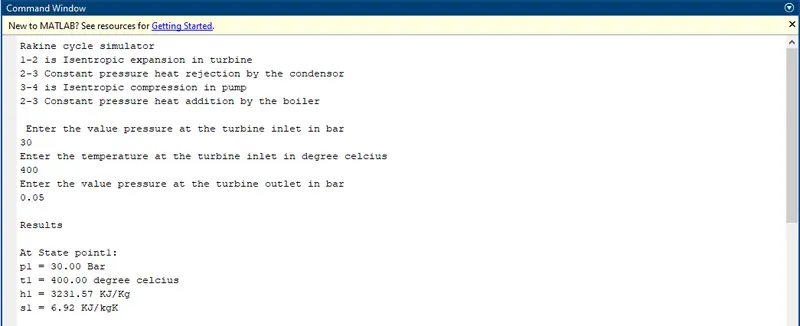
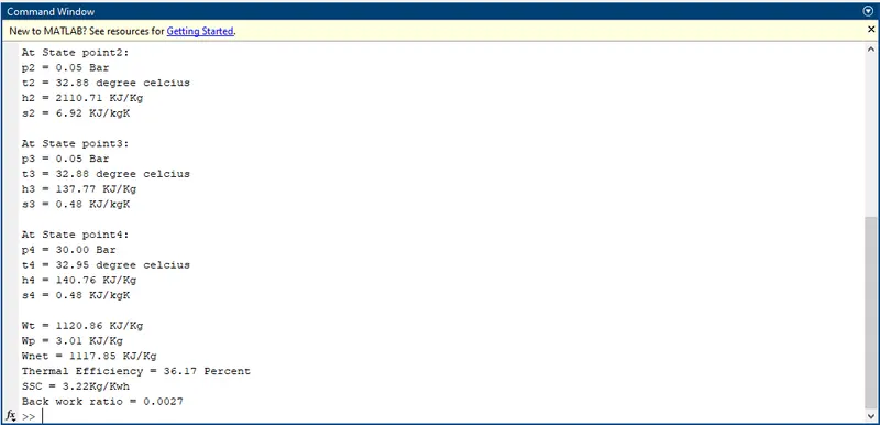
Output of state parameters of rankine cycle displayed in the command window :

Conclusion :

• The code is successfully compiled and the state parameters of a rankine cycle for a given set of user inputs is successfully calculated.
• The graphs for T-S and H-S of a rankine cycle is successfully plotted.
• The net work output and the back work ratio is successfully calculated.