Week 9 - FVM Literature Review
Objective :
To define about finite Volume Method(FVM), and to differentiate FDM & FVM and also to describe the need for interpolation schemes and flux limiters in FVM.
Finite difference method(FDM) :
- Finite Difference Method (FDM) is one of the methods used to solve differential equations that are difficult or impossible to solve analytically.
- In finite difference method the grids are linear and aligned so that all grid points are lie in a straight line and also the properties are consider to be concentrated at single point.
Finite volume method(FVM) :
- In finite volume method is applied over a volume so that the governing equation is valid over a entire volume and the properties are assumed to be concentrated at the geometric centre of the volume concerned.
Drawbacks of finite difference method :
- We cannot use it directly when the grids are not aligned along x,y and z direction since it has some complex folds and also the structure is complex. Because of unaligned grid points we can't able to calculate the properties at the next point exactly.
- In order to calculate the property approximately we need to introduce some correction term which is a correction factor.
- Introducing correction factor is tedious in case of complex geometry and this method of calculating the properties is called variable transformation method.
- Variable transformation method basically seeks to create a grid using a different variable space something like 'a' and 'b'. In 'a' and 'b' space the grid looks very similar to the cartesian grid and then suitable mapping function are defined which actually takes back to the orginal co-ordinates.
a,b <=> x,y
- If we can able to define a funtion like this we can take a fovering equation and write it interms of 'a' and 'b' and solve those equations then use variable transformation function to map the results back to the original grid. Creating these types of maps is going to be very hard when geometry becomes more complex.
Drawbacks of finite volume method :
The approach is as follows
- Divide space into numerous contiguous non-overlapping domains called cells.
- Integrate the equations of interest over the volume of each cell.
- For terms in the equations which dont involve spatial derivatives; this gives some form of average value associated with the cell centre.
- For terms which have spatial derivatives such as the divergence (transport) term, Gauss’ theorem can be used to convert this into an equivalent flux term.
This generates a discretised version of the equations. We do need to calculate the fluxes; on a colocated grid we interpolate values from the cell centres to do this. The big advantage of all this is that the cells can be any shape desired; this is a general method to derive the discretisation. I think it gets used in CFD because there is an intuitive interpretation of the result in terms of flows into and out of the cells.
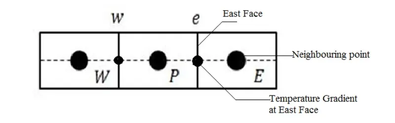
For examples consider 1-D Heat equation
`( (∂)/( ∂x))(( alpha.∂T)/( ∂x))+S =0`
`int( (∂)/( ∂x))(( alpha.∂T)/( ∂x))dv+Sdv =0`
`int( (∂)/( ∂x))(( alpha.∂T)/( ∂x))dv+intSdv =0` ---------> eqn 1.
generally `int(∂f)/(∂x) = f`
Therfore from eqn 1
`[ ( alpha.A.∂T)/( ∂x)]_w^e + overline S.dv` [dv = A.dx]
`( alpha_e.A.(T_E-T_P))/( dx) -( alpha_w.A.(T_P-T_w))/( dx) + overline S.dv`
`( alpha_e.A.(T_E-T_P))/( dx) -( alpha_w.A.(T_P-T_w))/( dx) + S_u+S_pT_p.dv`
- From the above equation we can say that the amount of heat that is removed from a particular box is concerned and even in a discritized form.
Gradint scheme :
- While calculating temperature we are calculating the temperature from the neighbouring points which is the points at the east and the west face is called gradient scheme.
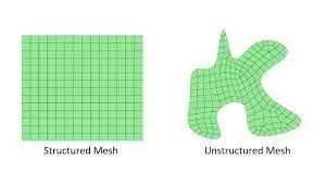
- The discretisation of the gradient operator is an important aspect of finite volume methods that has not received as much attention as the discretisation of other terms of partial differential equations. The most popular gradient schemes are the divergence theorem (or Green-Gauss) scheme, and the least-squares scheme. Both schemes are generally believed to be second-order accurate, but the present study shows that in fact the divergence theorem gradient is second-order accurate only on structured meshes whereas it is zeroth-order accurate on general unstructured meshes, and the least-squares gradient is second-order and first-order accurate, respectively.
Interpolation scheme :
The approximation of surface and volume integrals require the values of variables at locations other than the computational nodes of the control volume this could be found by using an interpolation scheme.
Various interpolation schemes are
- Upwind interpolation (UDS)
- Linear interpolation (CDS)
- QUICK
- Hybrid
- TVM
- ENO
1. Upwind interpolation (UDS) :
Upwind interpolation scheme depends on the direction of flow and it is mostly used for convection dominated problems.
If the flow is from W to E we used forward difference approximation and then the value of variable 'f' at the east face(e) is given by
`f_e = f_P`
If the flow is from E to W we used backward difference approximation and then the value of variable 'f' at the east face(e) is given by
`f_e = f_P` if `(v.n)_e > 0`
`f_e = f_E` if `(v.n)_e < 0`
Characteristics of upwind interpolation scheme :
- Upwind interpolation is the only interpolation which satisfies the boundedness criteria unconditionally irrespective of velocity and grid size.
- UDS is numerically diffusive this could be appropriated by the introduction numerical diffusive co-efficient.
- First order accurate hence very accurate grids are required to produce accurate solutions.
2. Linear interpolation (CDS) :
Linear interpolation is based on approximating the value of variables at the face center by using a central difference approximation for the first order derivative.
It takes two nearest compuatitional nodes for linear interpolation.
`f_e = f_Elamda_e + f_P(1-lamda_e)`
where as `lamda_e = (x_e -xp)/(x_E- x_P)`
Characteristics of linear interpolation :
- It is the simplest interpolation technique.
- Approximations are second order accurate for uniform grids and first order accurate for non-uniform grids.
- It may produce oscillatory solutions so small grids are preferred.
3. Quadratic upwind interpolation :
Quadratic upwind interpolation is based on approximating the value of variables at the face center by using a quadratic interpolation.
It requires three nearest computational nodes which is two upstream nodes and one downstream nodes.
`f_e = f_U + g_1(f_D - f_U) +g_2(f_(UU) - f_U)`
`g_1 = ((x_e -x_U)(x_e - x_(UU)))/((x_D -x_U)(x_D -x_(UU))`
`g_2 = ((x_e -x_U)(x_e - x_D))/((x_(UU) -x_U)(x_(UU)-x_D)`
Characteristics of quadratic interpolation :
- It is also most widely used in convection domination problems.
- Approximations are third order accurate for both uniform grids and non-uniform grids.
4. Hybrid interpolation scheme :
This scheme is the combination of both CDS and UDS based on the peclet number.
Flux limiters :
For convective fluid flow, it has been observed that low-order schemes are usually stable but quite dissipative in nature around points of discontinuity.
Higher order schemes are unstable in nature and show oscillations in the vincinity of discontinuity. Highly accurate and oscillation free schemes are known as high resolution schemes.
Flux limiter functions are used to tune higher order and lower schemes in such a way that the resulting scheme gives a higher order accuracy in the smooth region of the flow and maintains first order accuracy in the vincinity of shocks and discontinuities. For such a scheme the TVD(Total variation diminishing) criteria is maintained. Their basic forms are shown below.
`F(u_i+1/2) = f^(low)(i+1/2) -phi(r_i)(f^(low)(i+1/2)-f^(high)(i+1/2))`
`F(u_i-1/2) = f^(low)(i-1/2) -phi(r_i-1)(f^(low)(i-1/2)-f^(high)(i-1/2))`
where `f^(low)` = low precision flux(1st order accurate)
`f^(high)` = high precision flux(higher order accurate)
`phi(r)` = flux limiter function where r = `(u_i - u_(i-1))/(u_(i+1)-u_i)`