Week 4.1 - Genetic Algorithm
Aim :
To write a code in MATLAB to optimise the stalagmite function and to find the global maxima of that function.
Objective :
- To study about genetic algorithm.
- To study about the usage of genetic algorithm in MATLAB.
- To optimise the stalagmite function and to find the global maxima of that function.
Governing Equations :
Stalagmite function :
`f(x,y) = f1,x+f1,y+f2,x+f2,y`
`f1,x = [sin(5.1pix +0.5)]^6`
`f1,y = [sin(5.1piy +0.5)]^6`
`f2,x = exp[-4ln(2)(x-0.0667)^2/0.64]`
`f2,y = exp[-4ln(2)(y-0.0667)^2/0.64]`
where X and Y are the co-ordinates.
Gentic Algorithm syntax :
[inputs, fopt] = ga(@func,nvar,A,B,Aeq,Beq,lb,ub,nonlcon,Intcon,options)
func – function.
nvars – Number of variables.
A – Linear inequalities constraints.
B – Linear inequalities constraints.
Aeq - Linear equalities constraints.
Beq- Linear equalities constraints.
ub- upper bounds.
lb- lower bounds.
nonlcon – non linear constraints.
Intcon – Integer constraints.
Options – performs additional opertation like increasing populationsize.
Theory :
Genetic Algorithm :
A genetic algorithm is a search heuristic that is inspired by Charles Darwin’s theory of natural evolution. It is a method for solving both constrained and unconstrained optimization problems that is based on natural selection, the process that drives biological evolution.
Gentic Algorithm terminology :
Fitness Functions :
The fitness function is the function that we want to optimize. The fitness function determines how fit an individual is (the ability of an individual to compete with other individuals). It gives a fitness score to each individual. The probability that an individual will be selected for reproduction is based on its fitness score.
Individual :
An individual is any point to which you can apply the fitness function. The value of the fitness function for an individual is its score. For example, if the fitness function is
f(x1,x2,x3)=(2x1+1)2+(3x2+4)2+(x3−2)2,
the vector (2, -3, 1), whose length is the number of variables in the problem, is an individual. The score of the individual (2, –3, 1) is f(2, –3, 1) = 51.
An individual is sometimes referred to as a genome and the vector entries of an individual as genes.
Populations and Generations :
A population is an array of individuals. For example, if the size of the population is 100 and the number of variables in the fitness function is 3, you represent the population by a 100-by-3 matrix. The same individual can appear more than once in the population. For example, the individual (2, -3, 1) can appear in more than one row of the array.
At each iteration, the genetic algorithm performs a series of computations on the current population to produce a new population. Each successive population is called a new generation.
Diversity :
Diversity refers to the average distance between individuals in a population. A population has high diversity if the average distance is large; otherwise it has low diversity. In the following figure, the population on the left has high diversity, while the population on the right has low diversity.
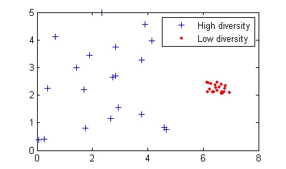
Diversity is essential to the genetic algorithm because it enables the algorithm to search a larger region of the space.
Fitness Values and Best Fitness Values :
The fitness value of an individual is the value of the fitness function for that individual. Because the toolbox software finds the minimum of the fitness function, the best fitness value for a population is the smallest fitness value for any individual in the population.
Parents and Children :
To create the next generation, the genetic algorithm selects certain individuals in the current population, called parents, and uses them to create individuals in the next generation, called children. Typically, the algorithm is more likely to select parents that have better fitness values.
Working of Genetic Algorithm :
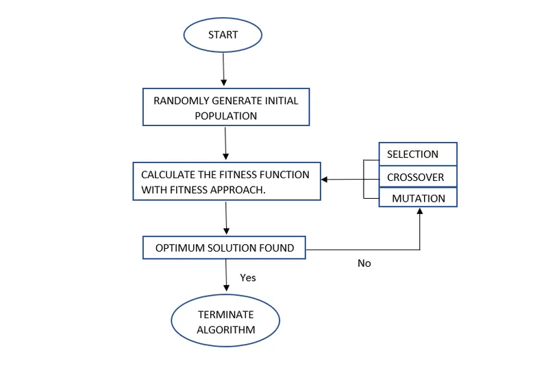
- The genetic algorithm selects individuals at random from the current population to be parents and uses them to produce the children for the next generation.
- This algorithm reflects the process of natural selection where the fittest individuals are selected for reproduction in order to produce offspring of the next generation.
- The fittest individuals are found based on the fitness function value.
- Over successive generations, the population "evolves" toward an optimal solution.
The genetic algorithm uses three main types of rules at each step to create the next generation from the current population:
- Selection rules select the individuals, called parents, that contribute to the population at the next generation.
- Crossover rules combine two parents to form children for the next generation.
- Mutation rules apply random changes to individual parents to form children.
Selection :
The idea of selection phase is to select the fittest individuals and let them pass their genes to the next generation.Two pairs of individuals (parents) are selected based on their fitness scores. Individuals with high fitness have more chance to be selected for reproduction.
Crossover :
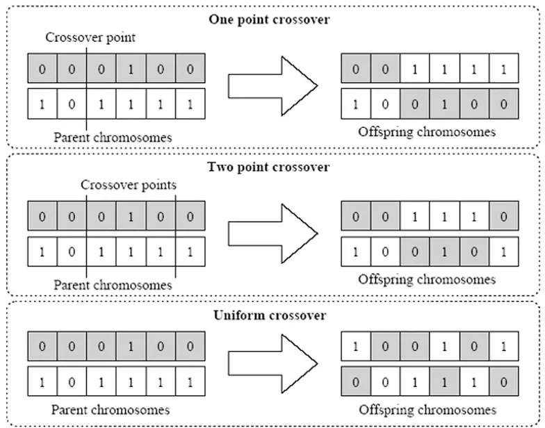
It is the process of taking two parents and producing the childs from them by interchanging the genes. There are three major types of crossover
Single point crossover :
A point on both parent chromosome are picked randomly and designated to be a crossover point.
Two-point crossover :
Two point on both parent chromosome are picked randomly and designated to be a crossover point.
Uniform crossover :
In a uniform crossover, typically, each bit is choosen from either parents with equal probability. The new offspring is added to the population.
Mutation :
It is the process of making random changes to the parents in order to maintain the genetic diversity. Mutation is consider as a secondary search operator for ga whereas crossover is consider as an primary search operator. There are many ways to perform mutation one of the way is bit flipped mutation.
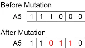
The other ways are swap mutation, insertion mutation and so on.
Note :
If the mutation is not performed, the chromosomes will become too similar to each other, converges takes place soon and the result in local minima.
Termination conditions :
- When there has been no improvement in the population for X-number of generations.
- When we reach an absolute number of generations.
- When the objective value has reached a certain predefined value.
Program :
Main program :
clear all
close all
clc

x = linspace(0,0.6,150);
y = linspace(0,0.6,150);

% creating 2-D mesh
[xx yy] = meshgrid(x,y);

% Evaluating the stalagmite function
for i=1:length(xx)
    for j=1:length(yy)
        input(1) = xx(i,j);
        input(2) = yy(i,j);
        f(i,j) = stalagmite(input);
    end
end
tic

% Case:1 - Statistical behaviour
numcases = 100
for i = 1:numcases
    [input,Fopt(i)] = ga(@stalagmite,2);
    xopt(i) = input(1);
    yopt(i) = input(2);
end
studytime1 = toc
figure(1)
subplot(2,1,1)
hold on
surfc(x,y,f);
shading interp
plot3(xopt,yopt,Fopt,'marker','o','markersize',5,'markerfacecolor','r')
title('Unbounded inputs')
subplot(2,1,2)
plot(Fopt)
xlabel('Iterations')
ylabel('function minimum')
fprintf('Study 1 statistical behaviour for unbounded inputs \n')
fprintf('Study time1 = %f \n',studytime1)
fprintf('The plot of global maxima is %f,%f\n',input(1),input(2))
fprintf('The functional value of global maxima is %f\n',(-mean(Fopt)))


% Case:2 - Statistical behaviour with upper and lower bounds
tic
for i = 1:numcases
    [input,Fopt(i)] = ga(@stalagmite,2,[],[],[],[],[0;0],[1;1]);
    xopt(i) = input(1);
    yopt(i) = input(2);
end
studytime2 = toc
figure(2)
subplot(2,1,1)
hold on
surfc(x,y,f);
shading interp
plot3(xopt,yopt,Fopt,'marker','o','markersize',5,'markerfacecolor','r')
title('Bounded inputs')
subplot(2,1,2)
plot(Fopt)
xlabel('Iterations')
ylabel('function minimum')
fprintf('Study 2 Statistical behaviour with upper and lower bounds \n')
fprintf('Study time2 = %f \n',studytime2)
fprintf('The plot of global maxima is %f,%f\n',input(1),input(2))
fprintf('The functional value of global maxima is %f\n',(-mean(Fopt)))


% Case:3 - Statistical behaviour with upper and lower bounds with increasing the GA iterations
tic

options = optimoptions('ga')
options = optimoptions(options,'populationsize',750);
for i = 1:numcases
    [input,Fopt(i)] = ga(@stalagmite,2,[],[],[],[],[0;0],[1;1],[],[],options);
    xopt(i) = input(1);
    yopt(i) = input(2);
end
studytime3 = toc
figure(3)
subplot(2,1,1)
hold on
surfc(x,y,f);
shading interp
plot3(xopt,yopt,Fopt,'marker','o','markersize',5,'markerfacecolor','r')
title('Bounded inputs')
subplot(2,1,2)
plot(Fopt)
xlabel('Iterations')
ylabel('function minimum')
fprintf('Study 3 Statistical behaviour with upper and lower bounds with increasing the GA iterations \n')
fprintf('Study time3 = %f \n',studytime3)
fprintf('The plot for global maxima is %f,%f\n',input(1),input(2))
fprintf('The functional value for global maxima is %f\n',(-mean(Fopt)))
Sub program :
function [F] = stalagmite(input)
  x = input(1);
  y = input(2);

  f1x = (sin(5.1*pi*x+0.5))^6;
  f1y = (sin(5.1*pi*y+0.5))^6;
  f2x = exp((-4)*log(2)*((x-0.0667)^2)/0.64);
  f2y = exp((-4)*log(2)*((y-0.0667)^2)/0.64);
  F = -f1x*f1y*f2x*f2y;
end
Program explanation :
- Firstly assign the values for x and y coordinates which varies from 0 to 0.6 at the interval of 150 using linspace command.
- Then create a 2-D mesh using meshgrid command.
- Seperately create a stalagmite function which is called as a sub program.
- Then call the stalagmite function in the main program inside a loop in order to generate stalagmites.
- The results of functional value has negative sign in order to find a global maxima.
Case 1 :
- In this case we made a study on statistical behaviour of genetic algorithm for unbounded inputs.
- This is done by assigning number of iterations.
- For our study we assigned numcases is equal to 100 which means it undergoes 100 iterations.
- The syntax used is [input,Fopt] = ga(@func,nvars)
func – function.
nvars – Number of variables.
- In our case stalagmite is our function and the number of variables is 2 which is x and y.
- In this case we just called a function it will calculate and gives the results of the coordinates and the functional value but we didn’t define any boundries because of this we wont get an optimum result.
- Tic and toc command used in this program is used to calculate the program running time for case 1.
- Assign case1 results as figure1 using figure command.
- Then plot the result of a stalagmite function using surfc command.
- Again plot the results such as xopt,yopt and fopt which is nothing but our calculated coordinates and the functional value using plot3 command and marker command by giving the appropriate markersize and marker face color. Plot3 command is used to made a 3-D plot.
- Hold on command is used to hold on the results in a same figure.
- Then plot the fopt value in order to find where exactly the global maxima is lies.
Case 2 :
- In this case we study about statistical behaviour of genetic algorithm for bounded inputs.
- This case is also same as that of case1 the only difference we will give upper and lower limits in order to define a search space.
- Because of this the syntax is modified as shown below
- [input,Fopt] = ga(@func,nvar,A,B,Aeq,Beq,lb,ub)
A – Linear inequalities constraints.
B – Linear inequalities constraints.
Aeq - Linear equalities constraints.
Beq- Linear equalities constraints.
ub- upper bounds
lb- lower bounds
- In our case we don’t have any equalities and inequalities so just give a blank bracket [].
- Where [0;0] & [1;1] are the lower and upper bounds respectively.
- The remaining steps are same as that of case 1.
Case 3 :
- In this case we made a study on statistical behaviour of genetic algorithm for bounded inputs with increase in population size.
- The syntax is modified as shown below,
- [input,Fopt] = ga(@func,nvar,A,B,Aeq,Beq,lb,ub,nonlcon,Intcon,options)
- func,nvars,A,B,Aeq,Beq,lb,ub are same as that case 1 and case 2.
nonlcon – non linear constraints
Intcon – Integer constraints.
Options – Used to increase the population size.
- In our case we don’t have any non linear and integer constraints so put blank bracket [].
- Options is used to increase the populationsize using optimoptions command in that give the appropriate populationsize in our case our populationsize is 750.
- It means it undergoes 750 iterations.
- The remaining procedures are same as that of case1 and case2.
Results :
Case 1 :
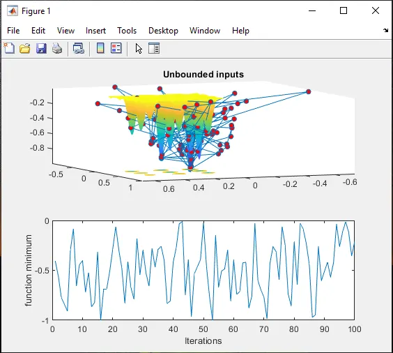
fig (1)

fig (2)
- fig (1) displays two graphs. The above graph is the graph plotted between coordinates(xopt,yopt) and the functional value(fopt).
- Our objective is to plot a global maxima but in that figure it is clear the plots are plotted randomly even outside the boundries.
- In the same fig (1) the graph below is the graph plotted between number of iterations and the functional value In that figure our global maxima varies in a wide range we cannot say where exactly the global maxima lies. From this we can conclude that the results are not much optimised.
- In this case we didnt define the boundries in order to get an optimised result we need to define a search space where the global maxima lies.
- Fig (2) displays the results of case 1 which is nothing but our studytime, coordinates and the functional value for case1.
Case 2 :
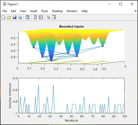
fig (3)

fig (4)
- fig (3) displays two graphs. The above graph is the graph plotted between coordinates(xopt,yopt) and the functional value(fopt).
- In that figure we can see that the results are much optimised when compare to that of case1 but the only thing is it lies in some local maxima's.
- In the same fig (3) the graph below is the graph plotted between number of iterations and the functional value. In that figure the functional values are some out clear and optimised when compare to that of case1.
- In this case the results are optimised when compare to that of case1 in order to get more accurate results we need to increase the number of iterations which is nothing but a populationsize.
- Fig (4) displays the results of case2 which is nothing but our studytime, coordinates and the functional value for case2.
Case 3 :
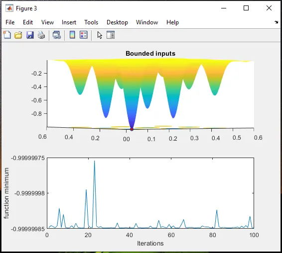
fig (5)

fig (6)
- fig (5) displays two graphs. The above graph is the graph plotted between coordinates(xopt,yopt) and the functional value(fopt).
- In that figure we can see that the results are optimised and the global maxima is displayed.
- In the same fig (5) the graph below is the graph plotted between number of iterations and the functional value. In that figure the functional values are clear and optimised.
- Fig (6) displays the results of case3 which is nothing but our studytime, coordinates and the functional value for case3.
Conclusion :
- The global maxima for the given stalagmite function is successfully optimized and compiled using genetic algorithm in matlab.
- The results are discussed above and the global maxima point lies in (0.066831,0.066832,1) which is our x,y,and z coordinates respectively.
Reference :
https://in.mathworks.com/help/gads/what-is-the-genetic-algorithm.html
https://www.tutorialspoint.com/genetic_algorithms/genetic_algorithms_fundamentals.htm
https://mech.iitm.ac.in/nspch52.pdf
https://skill-lync.com/knowledgebase/genetic-algorithm-explained
https://en.wikipedia.org/wiki/Genetic_algorithm
Project link :
https://skill-lync.com/student-projects/genetic-algorithm-188