Week 3.5 - Deriving 4th order approximation of a 2nd order derivative using Taylor Table method

Aim :

To derive the following 4th order approximations of the second-order derivative for central difference, skewed right-sided difference and skewed left-sided difference scheme.

Objective :

• To derive the following 4th order approximations of the second-order derivative for central difference, skewed right-sided difference and skewed left-sided difference and to prove that your skewed right-sided difference schemes of fourth-order approximation is accurate.
• To write a program in Matlab to evaluate the second-order derivative of the analytical function exp(x)*cos(x) and compare it with the 3 numerical approximations that we have derived.
• To provide a plot that compares the absolute error between the above-mentioned schemes and to dicuss about the needs of skewed scheme over a central differencing scheme skewed.

Taylor table for vaious scheme's :

Central differencing scheme :

calculation of number of nodes :

number of nodes = p+q-1

where as p is the order of approximation

q is the order of derivative.

number of nodes = 4+2-1

number of nodes = 5.

so,

`(∂^2phi)/(∂x^2) = (f(i-2)+f(i-1)+f(i)+f(i+1)+f(i+2))/(Δx^2)`

Taylor table,

.	`f(i)`	`f^'(i)Δx`	`f^('')(i)Δx^2`	`f^(''')(i)Δx^3`	`f^('''')(i)Δx^4`	`f^(''''')(i)Δx^5`	`f^(''''')(i)Δx^6`
`f(i-2)`	a	-2a	`(4a)/(2)`	`(-8a)/(6)`	`(16a)/(24)`	`(-32a)/(120)`	`(64a)/(720)`
`f(i-1)`	b	-b	`(b)/(2)`	`(-b)/(6)`	`(b)/(24)`	`(-b)/(120)`	`(-b)/(720)`
`f(i)`	c	0	0	0	0	0	0
`f(i+1)`	d	`d`	`(d)/(2)`	`(d)/(6)`	`(d)/(24)`	`(d)/(120)`	`(d)/(720)`
`f(i+2)`	e	`2e`	`(4e)/(2)`	`(8e)/(6)`	`(16e)/(24)`	`(32e)/(120)`	`(32e)/(720)`
sum	0	0	1	0	0	?	?

`a+b+c+d+e = 0`

`-2a-b+d+2e = 0`

`2a+(b)/(2)+(d)/(2)+e = 1`

`(-8a)/(6)+(-b)/(6)+(d)/(6)+(8e)/(6) = 0`

`(16a)/(24)+(b)/(24)+(d)/(24)+(16e)/(24) = 0`

AX = B

`((1,1,1,1,1),(-2,-1,0,1,2),(2,1/2,0,1/2,2),(-8/6,-1/6,0,1/6,8/6),(16/24,1/24,0,1/24,16/24))((a),(b),(c),(d),(e)) = ((0),(0),(1),(0),(0))`

X = `A^-1B`

X = `((-0.0833),(1.3333),(-2.5),(1.3333),(-0.0833))`

a = -0.0833, b = 1.3333 , c = -2.5, d = 1.3333, e = -0.0833.

`(∂^2phi)/(∂x^2) = (f(i-2)+f(i-1)+f(i)+f(i+1)+f(i+2))/(Δx^2)`

skewed right differencing scheme :

calculation of number of nodes :

number of nodes = p+q

where as p is the order of approximation

q is the order of derivative.

number of nodes = 4+2

number of nodes = 6.

so,

`(∂^2phi)/(∂x^2) = (f(i)+f(i+1)+f(i+2)+f(i+3)+f(i+4)+f(i+5))/(Δx^2)`

Taylor table,

.	`f(i)`	`f^'(i)Δx`	`f^('')(i)Δx^2`	`f^(''')(i)Δx^3`	`f^('''')(i)Δx^4`	`f^(''''')(i)Δx^5`	`f^(''''')(i)Δx^6`
`f(i)`	a	0	0	0	0	0	0
`f(i+1)`	b	b	`(b)/(2)`	`(b)/(6)`	`(b)/(24)`	`(b)/(120)`	`(-b)/(720)`
`f(i+2)`	c	2c	`(4c)/(2)`	`(8c)/(6)`	`(16c)/(24)`	`(32c)/(120)`	`(64c)/(720)`
`f(i+3)`	d	`3d`	`(9d)/(2)`	`(27d)/(6)`	`(81d)/(24)`	`(243d)/(120)`	`(729d)/(720)`
`f(i+4)`	e	`4e`	`(16e)/(2)`	`(64e)/(6)`	`(256e)/(24)`	`(1024e)/(120)`	`(4096e)/(720)`
`f(i+5)`	`f`	`5f`	`(25f)/2`	`(125f)/(6)`	`(625f)/(24)`	`(3125f)/(120)`	`(15625f)/(720)`
sum	0	0	1	0	0	0	?

`a+b+c+d+e+f= 0`

`b+2c+3d+4e+5f = 0`

`(b)/(2)+(4c)/(2)+(9d)/(2)+(16e)/(2)+(25f)/(2) = 1`

`(b)/(6)+(8c)/(6)+(27d)/(6)+(64e)/(6)+(125f)/(6) = 0`

`(b)/(24)+(16c)/(24)+(81d)/(24)+(256e)/(24)+(625f)/(24) = 0`

`(b)/(120)+(32c)/(120)+(243d)/(120)+(1024e)/(120)+(3125f)/(120) = 0`

AX = B

`((1,1,1,1,1,1),(0,1,2,3,4,5),(0,1/2,2,9/2,16/2,25/2),(0,1/6,8/6,27/6,64/6,125/6),(0,1/24,16/24,81/24,256/24,625/24),(0,1/120,32/120,243/120,1024/120,3125/120))((a),(b),(c),(d),(e),(f)) = ((0),(0),(1),(0),(0),(0))`

X = `A^-1B`

X = `((3.75),(-12.8333),(17.8333),(-13),(5.0833),(-0.0833))`

a = 3.75, b = -12.8333 , c = 17.8333, d = -13, e = 5.0833, f = -0.0833.

`(∂^2phi)/(∂x^2) = (f(i)+f(i+1)+f(i+2)+f(i+3)+f(i+4)+f(i+5))/(Δx^2)`

skewed left differencing scheme :

calculation of number of nodes :

number of nodes = p+q

where as p is the order of approximation

q is the order of derivative.

number of nodes = 4+2

number of nodes = 6.

so,

`(∂^2phi)/(∂x^2) = (f(i-5)+f(i-4)+f(i-3)+f(i-2)+f(i-1)+f(i))/(Δx^2)`

Taylor table,

.	`f(i)`	`f^'(i)Δx`	`f^('')(i)Δx^2`	`f^(''')(i)Δx^3`	`f^('''')(i)Δx^4`	`f^(''''')(i)Δx^5`	`f^(''''')(i)Δx^6`
`a(i-5)`	`a`	`-5a`	`(25a)/2`	`(-125a)/(6)`	`(625a)/(24)`	`(-3125a)/(120)`	`(15625a)/(720)`
`b(i-4)`	b	`-4b`	`(16b)/(2)`	`(-64b)/(6)`	`(256b)/(24)`	`(-1024b)/(120)`	`(4096b)/(720)`
`c(i-3)`	c	`-3c`	`(9c)/(2)`	`(-27c)/(6)`	`(81c)/(24)`	`(-243c)/(120)`	`(729c)/(720)`
`d(i-2)`	d	-2d	`(4d)/(2)`	`(-8d)/(6)`	`(16d)/(24)`	`(-32d)/(120)`	`(64d)/(720)`
`e(i-1)`	e	-e	`(e)/(2)`	`(-e)/(6)`	`(e)/(24)`	`(-e)/(120)`	`(-e)/(720)`
`f(i)`	f	0	0	0	0	0	0
sum	0	0	1	0	0	0	?

`a+b+c+d+e+f= 0`

`-5a-4b-3c-2d-e = 0`

`(25a)/(2)+(16b)/(2)+(9c)/(2)+(4d)/(2)+(e)/(2) = 1`

`-(125a)/(6)-(64b)/(6)-(27c)/(6)-(8d)/(6)-(e)/(6) = 0`

`(625a)/(24)+(256b)/(24)+(81c)/(24)+(16d)/(24)+(e)/(24) = 0`

`-(3125a)/(120)-(1024b)/(120)-(243c)/(120)-(32d)/(120)-(e)/(120) = 0`

AX = B

`((1,1,1,1,1,1),(5,4,3,2,1,0),(25/2,16/2,9/2,2,1/2,0),(125/6,64/6,27/6,8/6,1/6,0),(625/24,256/24,81/24,16/24,1/24,0),(3125/120,1024/120,243/120,32/120,1/120,0))((a),(b),(c),(d),(e),(f)) = ((0),(0),(1),(0),(0),(0))`

X = `A^-1B`

X = `((-0.0833),(5.0833),(-13),(17.8333),(-12.8333),(3.75))`

a = -0.8333, b = 5.0833 , c = -13, d = 17.8333, e = -12.8333, f = 3.75.

`(∂^2phi)/(∂x^2) = (f(i-5)+f(i-4)+f(i-3)+f(i-2)+f(i-1)+f(i))/(Δx^2)`

Program :

Main program :

clear all
close all
clc

x = pi/3;
dx =  linspace(pi/4,pi/4000,40);

for i = 1:length(dx)
    central_difference_error(i) =fourth_order_approximation_cd(x,dx(i));
    skewed_right_error(i) = fourth_order_approximation_sr(x,dx(i));
    skewed_left_error(i) = fourth_order_approximation_sl(x,dx(i));
end

loglog(dx, central_difference_error,'b','marker','square')
hold on
loglog(dx,skewed_right_error,'r','marker','square')
hold on
loglog(dx, skewed_left_error,'g','marker','square')
legend('central difference error','skewed right error','skewed left error')
grid on

Sub program :

Cental difference scheme :

function out = fourth_order_approximation_cd(x,dx)
% numerical derivative for a simple mathematical function

% analytical function = exp(x)*cosx;
% analytical derivative
% f''(x) = -2exp(x)*sinx

analytical_derivative = -2*exp(x)*sin(x)

% numerical derivative 
a = -0.0833;
b = 1.3333;
c = -2.5;
d = 1.3333;
e = -0.0833;
% central differencing d^2f(x)/dx^2 = (f(x-2dx)+f(x+dx)+f(x)+f(x+dx)+f(x+2dx))/dx^2
 central_differencing = ((a*exp(x-2*dx)*cos(x-2*dx))+(b*exp(x-dx)*cos(x-dx))+(c*exp(x)*cos(x))+(d*exp(x+dx)*cos(x+dx))+(e*exp(x+2*dx)*cos(x+2*dx)))/dx^2
out = abs(analytical_derivative- central_differencing )
end

Skewed right scheme :

function out = fourth_order_approximation_sr(x,dx)
% numerical derivative for a simple mathematical function

% analytical function = exp(x)*cosx;
% analytical derivative
% f''(x) = -2exp(x)*sinx

analytical_derivative = -2*exp(x)*sin(x)

% numerical derivative 
a = 3.75;
b = -12.8333;
c = 17.8333;
d = -13;
e = 5.0833;
f = -0.8333;
% skewed right differencing d^2f(x)/dx^2 = (f(x)+f(x+dx)+f(x+2dx)+f(x+3dx)+f(x+4dx)+f(x+5dx))/dx^2
 skewed_right_differencing = ((a*exp(x)*cos(x))+(b*exp(x+dx)*cos(x+dx))+(c*exp(x+2*dx)*cos(x+2*dx))+(d*exp(x+3*dx)*cos(x+3*dx))+(e*exp(x+4*dx)*cos(x+4*dx))+(f*exp(x+5*dx)*cos(x+5*dx)))/dx^2
out = abs(analytical_derivative- skewed_right_differencing )
end

Skewed left scheme :

function out = fourth_order_approximation_sl(x,dx)
% numerical derivative for a simple mathematical function

% analytical function = exp(x)*cosx;
% analytical derivative
% f''(x) = -2exp(x)*sinx

analytical_derivative = -2*exp(x)*sin(x)

% numerical derivative 
a = -0.8333;
b = 5.0833;
c =  -13;
d = 17.8333;
e = -12.8333;
f = 3.75;
% skewed left differencing d^2f(x)/dx^2 = (f(x)+f(x+dx)+f(x+2dx)+f(x+3dx)+f(x+4dx)+f(x+5dx))/dx^2
 skewed_left_differencing = ((a*exp(x-5*dx)*cos(x-5*dx))+(b*exp(x-4*dx)*cos(x-4*dx))+(c*exp(x-3*dx)*cos(x-3*dx))+(d*exp(x-2*dx)*cos(x-2*dx))+(e*exp(x-dx)*cos(x-dx))+(f*exp(x)*cos(x)))/dx^2
out = abs(analytical_derivative- skewed_left_differencing )
end

Program explanation :

• Firstly begin the code with clear all, close all and clc command. Clear all and close all command clears and closes the previously opened file and clc command is used to clear the command window.
• Then define the inputs such as variable x the point in which we need to compute the function which is at pi/3 and dx varies from pi/4000 to pi/4 in between these we need to get 40 values this is assigned by using linspace command.
• In this program we used three different functions to calculate the fourth order approximation of second order derivative using various schemes such as central differencing, skewed right differencing and skewed left differencing scheme respectively.
• Inside these function we are computing for both numerical value and the analytic value for the function `f(x) = e^(x)cosx` .
• In order to calculate the numerical value with fourth order approximation we used central differencing, skewed right differencing and skewed left differencing scheme respectively.
• The formula for this are computd using a taylor table method.
• Then difference in analytical and numerical value is the error parameter.
• The error parameter stores in the variable called 'out'. While calculating error we are using abs command in order to get an absolute value of an error which gives the accurate results.
• Then end key word is used to end the function.
• Then using for loop the subprograms which is functions to compute central differencing, skewed right differencing and skewed left differencing called inside the main program from these functions we get an output as error value with a fourth order approximations in each scheme. The size of loop is same as that of length of dx.
• Then plot the results between dx and error for various scheme which is central differencing, skewed left and skewed right in the form of plots using loglog command.
• loglog command is used to made a plot which defines x and y axis in a lograthimic scale in order get a plot efficiently.
• Then hold on command is used to hold on all the error plots of various order of derivatives in the same graph and name the this graph as figure(1) using figure command.
• Then name the x and y axis in the plots using xlabel and y label command.
• Finally lengends are provided to make our plots more detailed using legend command.

Output :

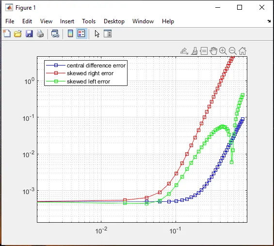
figure(1)

figure(1) shows the graph plotted between dx and the error which is generated using various schemes which is central differencung, skewed right, and schewed left scheme. From the plot it is clear that the error generated in central differencing scheme is less when compare to that of skewed right and the skewed left scheme eventhough the error generated in central differencing scheme is low we cannot use central differencing scheme in all situation. Suppose if we want to compute numerical approximation of a function in the boundary we can't able to use central differencing scheme since it requires input from both the sides in that case skewed scheme plays a vital role. In skewed scheme it requires data from one side to compute a numerical approximation at a point.

Conclusion :

The matlab code which compute both numerical and analytical value of a given function using various schemes is successfully compiled and the error generated in these schemes are compared using a graph. From graph it is clear that the error generated in central differencing scheme is minimum when compare to that of skewed right and skewed left schemes.