Curve Fitting

Aim :

To write a matalab program to perform curve fitting operation and to find the best fit for the given data set.

Objective :

• To plot linear fit and cubic polynomial fit for the given temperature and cp data along with the raw data points.
• To explain about the parameters used to measure the fitness characteristics for both the curves.
• To explain about the difference between the perfect fit and the best fit.
• To explain about how to increase the efficiency of the cubic fit curve.
• To explain the splitwise method of coding.

Theory :

Curve fitting :

Curve fitting is nothing but deriving equation from the set of available data points on the graph such that root mean square error of all predicted points is minimum. In other words, we try to derive the equation of curve such that it passes as closely as possible through all the given data points.

Types of curve used in curve fitting:

The first degree polynomial equation (Linear curve) :

`y= ax+b`

The second degree polynomial equation (Quadratic curve) :

`y= ax^2+bx+c`

The three degree polynomial equation (Cubic curve) :

`y = ax^3+bx^2+cx+d`

Parameters used to measure the fitness characteristic of the curve

While fitting a curve we will expect a best fit. Our ultimate aim is to identify the best fitted curve which satisfies the data points. There are 4 quantities which help us to measure the goodness of fit criteria or how well the equation is representing the data points. There are

1. Sum of square due to error
2. R-Square
3. Adjusted R-Square
4. Root mean squared error

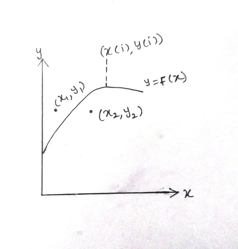
Sum of square due to error :

Sum of square due to error is the square of difference between the actual data point and the predicted data point.

Error = |y(i) - value of f(x) at x(i)|

= |y(i) - f(x(i))|

To remove the modulus sign, it is effective if we square the error term, when we square the error terms and add errors for all 'n' points we get

`SSE = sum_(i=1)^n`Error`(i)^2`

`SSE = sum_(i=1)^n(f(x(i)) -mean)^2`

The error should be minimum in order to get a good fit.

R-Square :

R-Square is the square of response value and the predicted response value. Higer value of R-Square will lead to best fit and the lower value of R-Square will leads to worst fit. Usually R-Square ranges from 0 to 1.

0 indicates the worst possible fit for the data set.

1 indicates the best possible fit for the data set.

`R^2 = (SSR)/(SST)`

`SSR = sum_(i=1)^n(y(i) - f(x(i)))^2`

SST = SSR + SSE

SSR - Sum of squares of regression

SSR - The square of the difference between the value of fitting fumction at a given point and the arithmetic mean of the data set.

Adjusted R-square :

It is a normalizing variation of R-Square which neglects the variation of R-square due to insignificant dependent variable.

Let y = f(x)

If the value of x(i) contribute to the output y, then x(i) is a significant dependent variable.

If the value of x(i) does not contribute to the output y, then x(i) is a insignificant dependent variable.

So, adjusted R-square disregards these infinitesmally small increments to R-Square and only considers the variables which actually contribute to the output of ths system in a drastic way.

`R_(adj)^2` = 1 - `[((1-R^2)(n-1))/((n-k-1))]`

`R_(adj)^2` equal to one or closer to one indicates a best fit of the curve.

Root Mean squared error(RSME) :

Root mean square error is a measure of difference between the actual curve and the predicted curve. It is the estimate of the standard deviation of the random component of the data.This statistic is also known as fit standard error or the standard error of regression.

RSME = `sqrt((SSE)/(n))`

RSME = `sqrt((sum_(i=1)^n(f(x(i)) -mean)^2)/(n))`

n - Total number of data points available.

RSME value closer to zero is consider to be a good fit.

Program :

clear all
close all 
clc

% preparing data
cp_data = load('data');
temperature = cp_data(:,1);
cp = cp_data(:,2);

% curve fitting

% Linear curve fitting
figure(1)
plot(temperature,cp,'linewidth',2)
hold on
coefficient_1 = polyfit(temperature,cp,1);
cp_predicted_1 = polyval(coefficient_1,temperature);
plot(temperature,cp_predicted_1,'linewidth',2)
xlabel('Temperature(K)')
ylabel('Specific heat(KJ/mol-k)')
title('Linear curve fit')
legend('Original cp','Linear curve fitting')

% cubic curve fitting

figure(2)
plot(temperature,cp,'linewidth',2)
hold on
coefficient_3 = polyfit(temperature,cp,3);
cp_predicted_3 = polyval(coefficient_3,temperature);
plot(temperature,cp_predicted_3,'linewidth',2)
xlabel('Temperature(K)')
ylabel('Specific heat(KJ/mol-k)')
title('Cubic curve fit')
legend('Original cp','Cubic curve fitting')

% parameters which is used to calculated the fitness characteristics
%For linear curve

% Mean cp
Total_cp = 0;
for i = 1:length(temperature)
    Total_cp = Total_cp + cp(i);
end
 mean = Total_cp/3200;

% SSR = (cp_predicted - mean)^2
SSR_3 = 0;
for j = 1:length(temperature)
    SSR_3 = SSR_3 + (cp_predicted_1(j)-mean)^2;
end

% SSE = (cp - cp_predicted)^2
SSE_3 = 0;
for k = 1:length(temperature)
    SSE_3 = SSE_3 + (cp(k) - cp_predicted_1(k))^2;
end

R_square_linear = SSR_3/(SSR_3+SSE_3)

if R_square_linear >= 0.95
    disp('R_square_linear is a good fit')
else
    disp('R_square_linear is not a good fit')
end

%For cubic curve

% Mean cp
Total_cp = 0;
for i = 1:length(temperature)
    Total_cp = Total_cp + cp(i);
end
 mean = Total_cp/3200;

% SSR = (cp_predicted - mean)^2
SSR = 0;
for j = 1:length(temperature)
    SSR = SSR + (cp_predicted_3(j)-mean)^2;
end

% SSE = (cp - cp_predicted)^2
SSE = 0;
for k = 1:length(temperature)
    SSE = SSE + (cp(k) - cp_predicted_3(k))^2;
end

R_square_cubic = SSR/(SSR+SSE)

if R_square_cubic >= 0.95
    disp('R_square_cubic is a good fit')
else
    disp('R_square_cubic is not a good fit')
end

Program explanation :

• Load the cp and temperature data using load command.
• Then store the loaded values in temperature and cp.
• In matlab curve fitting is performed using two functions polyfit and polyval.
• Polyfit is a Matlab function that computes a least squares polynomial for a given set of data. Polyfit generates the coefficients of the polynomial, which can be used to model a curve to fit the data.The co-efficients is generated according to degree of a polynomial that we are given.
• Polyval evaluates a polynomial for a given set of x values. So, Polyval generates a curve to fit the data based on the coefficients found using polyfit.
• The curve which is generated by the polyval command is our predicted curve.
• Then plot the original curve and predicted curve in the same figure in order to identify the difference between these two curves.
• Hold on command is used to hold both the curves in a same figure.
• In order to identify the curve which we predicted is a Best fit or not we need to calculate some parameters(SSE & R-Square). These parameters help us to identify the fitness characteristics of the curve.
• If the R-square value is greater than or equal to 0.95 then the curve is said to be a good fit.
• This process is repeated by changing the order of the polynomial until we get a best fit of the curve.
• The value which is closer or equal to 1 is said to be a best fit.

OUTPUT

:

Fig(1)

Fig(2)

Fig(3)

Explanation :

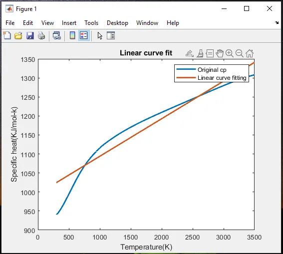
• Fig(1) is the graph indicates a orignal curve and the linear curve. The orignal curve is plotted by means of a raw data set and the linear curve is plotted by means of a predicted data set.
• From Fig(1) it is clear that the predicted curve does not match the original curve.
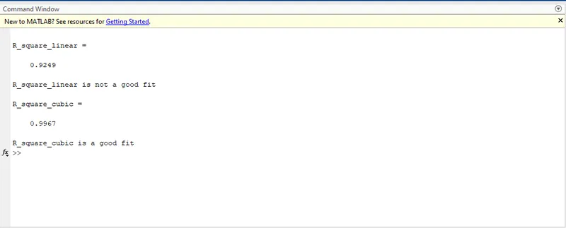
• Fig(1) is not said to be a best fit of the curve because the R_Square(fitness characteristics ) we have got was 0.9249 which is less than 0.95.
• The R-Square value which is above 0.95 is said to be a best fit.
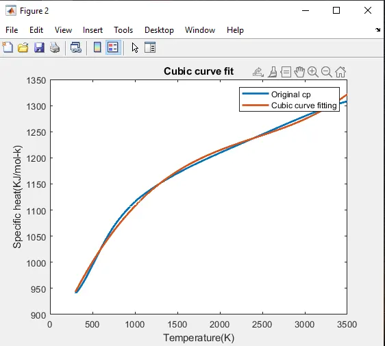
• Fig(2) is the graph indicates a orignal curve and the linear curve. The orignal curve is plotted by means of a raw data set and the cubic curve is plotted by means of a predicted data set.
• From Fig(2) the predicted curve is said to be a best fit because R-Square value of Cubic curve is 0.9967 from Fig(3) which is greater than 0.95.
• So the cubic curve is said to be a best fit.
• Even though we made a best fitted curve we always try to get the perfect fit.

The term Best fit and the perfect fit :

Best fit :

The difference between the actual measured value and the predicted value is minimum is said to be a best fit.

Perfect fit :

Perfect fit means the curve should fit the original curve without showing any errors (such as centering and scaling errors) in that particular degree of polynomial. Perfect fit can always be a best fit but the best fit cannot be a perfect fit.

In order to get a perfect fit we need to increase the order of the polynomial or we need to use the splitwise method. If we keep on increase the order of the polynomial which eventually leads to the overfitting. So splitwise method is preferred.

Split wise method :

In this method we can split the original data into small ranges by means of which we can compute a different co-efficients for the curve fit function for that small ranges. Finally we combine all these values we can able to plot a entire data set. Cubic fit is also get improved by this method.

Splitwise Program :

clear all
close all 
clc

% preparing data
cp_data = load('data');
temperature = cp_data(:,1);
cp = cp_data(:,2);

temperature_1 = cp_data(1:800,1);
temperature_2 = cp_data(801:1600,1);
temperature_3 = cp_data(1601:2400,1);
temperature_4 = cp_data(2401:3200,1);

cp = cp_data(:,2);
cp_1 = cp_data(1:800,2);
cp_2 = cp_data(801:1600,2);
cp_3 = cp_data(1601:2400,2);
cp_4 = cp_data(2401:3200,2);


% curve fitting

% Linear curve fitting
figure(1)
plot(temperature,cp,'linewidth',2)
hold on
coefficient_1 = polyfit(temperature_1,cp_1,2);
coefficient_2 = polyfit(temperature_2,cp_2,2);
coefficient_3 = polyfit(temperature_3,cp_3,2);
coefficient_4 = polyfit(temperature_4,cp_4,2);

cp_predicted_1 = polyval(coefficient_1,temperature_1);
cp_predicted_2 = polyval(coefficient_2,temperature_2);
cp_predicted_3 = polyval(coefficient_3,temperature_3);
cp_predicted_4 = polyval(coefficient_4,temperature_4);


plot(temperature_1,cp_predicted_1,'linewidth',3,'color','r')
hold on
plot(temperature_2,cp_predicted_2,'linewidth',3,'color','r')
hold on
plot(temperature_3,cp_predicted_3,'linewidth',3,'color','r')
hold on
plot(temperature_4,cp_predicted_4,'linewidth',3,'color','r')

xlabel('Temperature(K)')
ylabel('Specific heat(KJ/mol-k)')
title('cubic curve fit')
legend('Original cp','Cubic curve fitting')


% parameters which is used to calculated the fitness characteristics
%For cubic curve

cp_predicted = [cp_predicted_1;cp_predicted_2;cp_predicted_3;cp_predicted_4]

% Mean cp
Total_cp = 0;
for i = 1:length(temperature)
    Total_cp = Total_cp + cp(i);
end
 mean = Total_cp/3200;
 
% SSR = (cp_predicted - mean)^2
SSR = 0;
for j = 1:length(temperature)
    SSR = SSR + (cp_predicted(j)-mean)^2;
end

% SSE = (cp - cp_predicted)^2
SSE = 0;
for k = 1:length(temperature)
    SSE = SSE + (cp(k) - cp_predicted(k))^2;
end

R_square_cubic = SSR/(SSR+SSE)

if R_square_cubic >= 0.95
    disp('R_square_cubic is a good fit')
else
    disp('R_square_cubic is not a good fit')
end

Program explanation :

• The same procedure is followed that we mentioned in the above program the only difference is we are splitting a data into 4 rages.
• Because of that we will get a four different co-efficients.
• plot the original data set.
• Plot all the four different co-efficients along with the temperature ranges.
• Then calculate the fitness characteristics for that splited data and combine all the values and finally Calculate the R-Square value which will give the results whether the predicted curve is good fit or not.

OUTPUT :

Fig(4)

Fig(5)

Explanation :

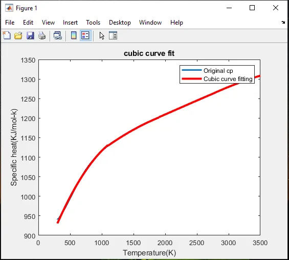
• Fig(4) is the graph indicates a orignal curve and the cubic curve plotted using the split wise method The orignal curve is plotted by means of a raw data set and the Cubic curve is plotted by means of a predicted data set.
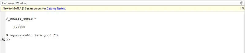
• From Fig(4) the predicted curve is said to be a perfect fit because R-Square value of Cubic curve is 1 from Fig(5) which means the predicated curve exactly matches the orginal curve there is no deviation in between these two curves.

Conclusion :

• The MATLAB program to perform curve fitting operation for linear and cubic curve is successfully compiled and the results of this program is shown above.
• From the above results we can say that the curve with higher degree polynomial equation will give the better fit. Splitwise method is suggested to use in order to get a maximum best result.

Reference :

https://en.wikipedia.org/wiki/Curve_fitting

https://skill-lync.com/knowledgebase/the-basic-concept-of-curve-fit

https://skill-lync.com/student-projects/Curve-Fitting-and-criterion-to-choose-best-fit-41860

https://skill-lync.com/knowledgebase/curve-fit-toolbox-an-overview