Solving 2nd order ODE of a simple pendulum using MATLAB

AIM :
To write a MATLAB program that will simulate the motion of the simple pendulum.

THEORY :

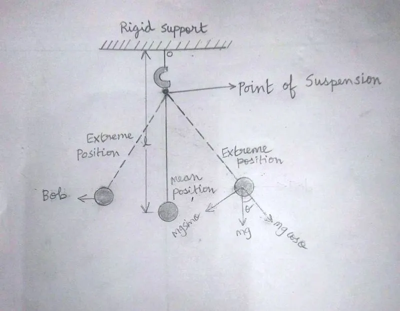
A heavy point mass (known as bob) suspended from a rigid support by a massless and inextensible string is called simple pendulum. The vertical line passing through the fixed support is the mean position of a simple pendulum.

The vertical distance between the point of suspension and the centre of mass of the suspended body (when it is in mean position) is called the length of the simple pendulum denoted by l.

These are important terms pertaining to simple pendulum:

• Oscillation of a simple pendulum : One complete to and fro motion of the pendulum is called one oscillation
• Time period of a simple pendulum : It is defined as the time taken by the pendulum to finish one full oscillation and is denoted by “T”.
• Frequency of oscillation : It is the number of oscillations made in one second.

ORDINARY DIFFERENTIAL EQUATIONS(ODE) :

An Ordinary Differential Equation is a differential equation that depends on only one independent variable.

For example,

`dy/dx = ky(t)`

It is an ordinary differential equation(First order) because y depends only on t(the independent variable).

SECOND ORDER DIFFERENTIAL EQUATION OF SIMPLE PENDULUM:

In general ODE is used to describe the transient behaviour of the system.

Example : Simple pendulum.

The position of the bob in the simple pendulum is examined by solving second order differential equation given below.

`(d^2theta)/(dt^2)+(b)/(m)(d theta)/(dt)+g/lsintheta = 0``rarr`eqn(1)

This can be achieved by breaking the second order ODE into two first order ODE’s.

CALCULATIONS :

`theta =theta_1`

`(d theta)/(dt)` = `(d theta_1)/(dt) = theta_2` `rarr`eqn(2)

put `theta = theta_1` in eqn(1)

eqn(1) `rArr``(d^2theta_1)/(dt^2)+(b)/(m)(d theta_1)/(dt)+g/lsintheta_1 = 0`

`(d)/(dt)((d theta_1)/(dt))+(b)/(m)(theta_2)+g/lsintheta_1 = 0`

`(d(theta_2))/(dt)+(b)/(m)(theta_2)+g/lsintheta_1 = 0`

`(d(theta_2))/(dt) = -(b)/(m)(theta_2)-g/lsintheta_1 ` `rarr`eqn(3)

Express this equation in the matrix form

`d/dt((theta_1),(theta_2)) = ((theta_2),(-(b)/(m)(theta_2)-g/lsintheta_1))`

NOTATION :

g – gravity in m/`s^2`

l – length of a pendulum in m.

m – mass of a ball in kg.

b – damping co-efficient.

PROGRAM :

MAIN PROGRAM :

clear all
close all 
clc

% Inputs
b = 0.05;
g = 9.81
l = 1
m = 0.1

% Initial Condition
theta_0 = [0;3];
t_span = linspace(0,20,500);

% Solve ODE
[t,results] = ode45(@(t,theta)ode_func(t,theta,b,g,l,m),t_span,theta_0);

figure(1)
plot(t,results(:,1))
hold on
plot(t,results(:,2))
xlabel('Angular displacement & Angular velocity')
ylabel('Time')
legend('Angular displacement','Angular velocity')

figure(2)
plot(results(:,1),results(:,2))
xlabel('Angular displacement in rad')
ylabel('Angular velocity in rad/sec')



% Animation
ct = 1
for i=1:length(t_span)
    X_initial = 0;
    Y_initial = 0;
    
    X_final = l*sin(results(i,1));
    Y_final = -l*cos(results(i,1));
    
    figure(3)
    plot([-1 1],[0 0],'linewidth',5,'color','r')
    hold on
    plot([0 0],[0 -1.5],'linewidth',5,'color','b')
    hold on
    plot([X_initial X_final],[Y_initial Y_final],'linewidth',2)
    hold on
    plot(X_final,Y_final,'marker','o','markersize',20,'markerfacecolor','r')
    hold off
    axis([-2 2 -2 1])
    grid on
   
    M(ct) = getframe(gcf);
    ct=ct+1
end
movie(M)
videofile = VideoWriter('pendulum_simulation','uncompressed AVI')
open(videofile)
writeVideo(videofile,M)
close(videofile)

SUB PROGRAM :

function [dtheta_dt] = ode_func(t,theta,b,g,l,m)
  theta1 = theta(1)
  theta2 = theta(2)
  dtheta1_dt = theta2
  dtheta2_dt = -(b/m)*theta2-(g/l)*sin(theta1)
  dtheta_dt = [dtheta1_dt; dtheta2_dt];
end  

PROGRAM EXPLANATION :

• Give inputs such as g, l, b, m, θ2(initial velocity), θ1(initial displacement), and t_span(time).
• t_span varies from 0 to 90 sec in between 0 to 90 sec we are getting 500 values for t_span using linspace command.
• Then we are using function the ODE solver which is ode45 is an inbuilt function present in the MATLAB in order to solve second order differential equation.
• The ode45 has fourth order Runge-kutta method for solving second order differential equation of simple pendulum.
• After solving this ode45 we will get the results of theta1 and theta2 which is our angular displacement and angular velocity.
• Then plot the results between Time VS Angular velocity & Angular displacement and then Angular velocity VS Angular displacement using plot command.
• For generating animation we are using for loop. For loop runs upto the length of t_span.
• One end of the pendulum is fixed so plot X_initial and Y_initial is equal to zero.
• X_final and Y_final is the final position of the simple pendulum is calculated by solving the equation X_final = l*sinθ & Y_final = -l*cosθ.
• Cos component is taken as negative because the pendulum oscillate along downwards or else in the negative y-direction.
• Then plot the blue line which will our mean point.
• Then plot the red line which will be our support.
• Then plot the X_final and Y_final value of a simple pendulum.
• At the end of the string of the simple pendulum we need a bob that can achieved by using marker command.
• Again plot X_final and Y_final value and use the marker command then give the appropriate markesize and marker face color.
• Then set the axis appropriately using axis command.
• Hold on command is used to hold all the plots that we have made in a single frame.
• After the frames are formed we need to capture these animation in the video.
• Each frame is captured in an array(M)then getframe(gcf) command is used to get these frames in an array.
• Then movie(M)command is used to create a movie using the frames captured in an array called M.
• Then give the file name and type of file using videofile.
• Then open the videofile using open(videofile)command then writeVideo command is used to write video in the videofile.
• Then close(vediofile)command is used to close the videofile.

OUTPUT :

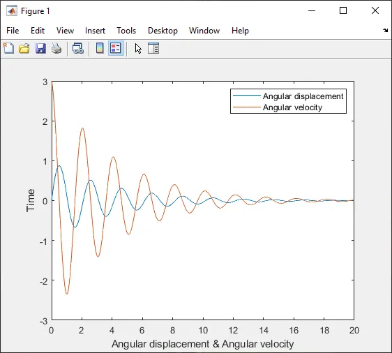
fig(1) Angular displacement &Angular velocity VS Time

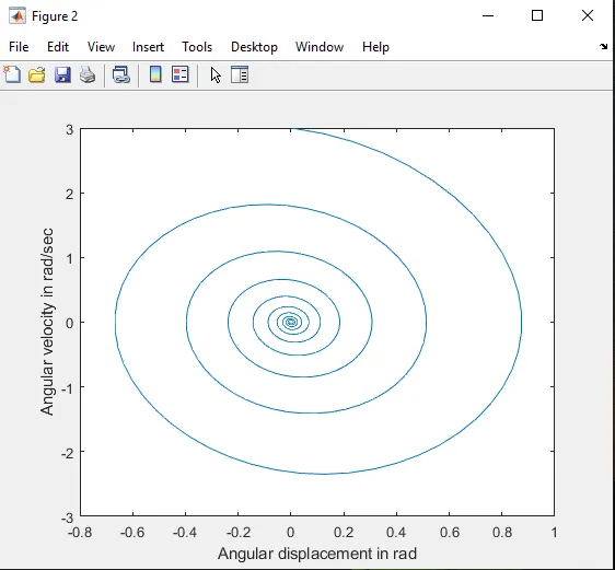
fig(2) Angular displacement VS Angular velocity

ANIMATION :

https://youtu.be/OF7w_KZOaf8

CONCLUSION :

• Fig(1) is the graph ploted between Time VS Angular velocity & Angular displacement. It shows that how Angular velocity and Angular displacement varies with respect to time.
• Fig(2) is the graph ploted between Angular velocity VS Angular displacement. It shows that how the angular position of the pendulum varies with respect to the angular velocity.
• A MATLAB program that will simulate the motion of the simple pendulum is successfully compiled and the simulated vedio link is attached with the output.