Week 5.1 - Mid term project - Solving the steady and unsteady 2D heat conduction problem
AIM:
To write the code which solves the 2D heat conduction equation by using the point iterative techniques by implementing the following methods.
1. Jacobi
2. Gauss-seidel
3. Successive over-relaxation
OBJECTIVES:
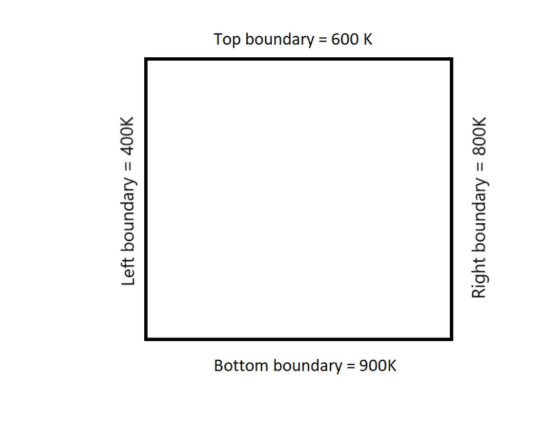
1. To solve the 2D heat conduction equation by using the point iterative techniques that were taught in the class. The Boundary conditions for the problem are as follows;
Top Boundary = 600 K
Bottom Boundary = 900 K
Left Boundary = 400 K
Right Boundary = 800 K
By implementing the following methods for solving implicit equations.
- Jacobi
- Gauss-seidel
- Successive over-relaxation
With absolute error criteria is 1e-4
2. To write code for both implicit and explicit schemes (This is for the transient analysis only)
3. Compare the convergence rate [Number of iterations] of the steady state and transient [explicit and implicit] simulations and justify the numerics.
PROCEDURE:
Domain is assumed to be a shape of a square of lenght 1m.
No. of nodes at x and y direction be nx=ny=10.
Temperature at the nodes,
- Top Boundary = 600 K
- Bottom Boundary = 900 K
- Left Boundary = 400 K
- Right Boundary = 800 K
- Initial temperature inside the domain=300 K
- Top left corner
- Top right corner
= (
- Bottom left corner
= (
- Bottom right corner
= (
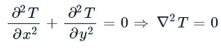
Steady state 2D heat conduction equation:
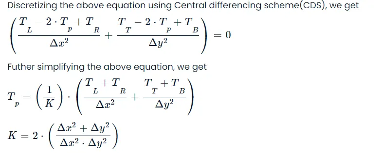
Jacobi method:
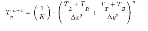
Gauss seidel method:
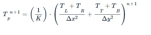
Successive over relaxation method or SOR method:

MATLAB CODE:
Steady State Analysis by IMPLICIT Method
% Steady state heat conduction by IMPLICIT Method

clear all
close all
clc

%initial conditions
%L = 1
nx = 10;
ny = 10;
x = linspace(0,1,nx);
y = linspace(0,1,ny);
dx = x(2) - x(1);
dy = y(2) - y(1);


% Boundary condition

t = 300*ones(nx,ny);
t(:,1) = 400;
t(1,:) = 600;
t(:,ny) = 800;
t(nx,:) = 900;

% defining the temperature at corner points

t(1,1) = 500;
t(nx,ny) = 850;
t(1,ny) = 700;
t(nx,1) = 650;

dt = 1e-2; %time step
told=t;

error = 100;
tol = 1e-4;
k = 2*(dx^2+dy^2)/(dx^2*dy^2);
% k2 = (dy^2)/(2*(dx^2+dy^2));

method = input('Iterative method = ');

%JACOBI ITERATIVE METHOD

if (method==1)
    tic;
    jacobi = 1;
    while(error>tol)
        for i = 2:(nx-1)
            for j = 2:(ny-1)
            t(i,j) = (((told(i-1,j)+told(i+1,j))/(dx^2))+((told(i,j+1)+told(i,j-1))/(dy^2)))/k;
            end
        end
    error = max(max(abs(t-told)));
    told = t;
    jacobi = jacobi+1;
    time_taken = toc;
    end

%plotting
figure(1)
contourf(x,y,t,'ShowText','on');
colormap(jet);
colorbar;
set(gca,'ydir','reverse')
xlabel('X')
ylabel('Y')
text1 = sprintf('number of iteration = %d', jacobi);
text2 = sprintf('simulation time = %f', time_taken);
title({'Steady state heat conduction by jacobi'; text1; text2});
end


%GAUSS-SEIDEL ITERATIVE METHOD

if (method==2)
    tic;
    gauss = 1;
    while(error>tol)
        for i = 2:(nx-1)
            for j = 2:(ny-1)
            t(i,j) = (((t(i-1,j)+told(i+1,j))/(dx^2))+((told(i,j+1)+t(i,j-1))/(dy^2)))/k;
            end
        end
    error = max(max(abs(t-told)));
    told = t;
    gauss = gauss+1;
    time_taken = toc;
    end

%plotting
figure(2)
contourf(x,y,t,'ShowText','on');
colormap(jet);
colorbar;
set(gca,'ydir','reverse')
xlabel('X')
ylabel('Y')
text1 = sprintf('number of iteration = %d', gauss);
text2 = sprintf('simulation time = %f', time_taken);
title({'Steady state heat conduction by Gauss-Seidel'; text1; text2});
end


%SUCCESSIVE OVER RELAXATION ITERATIVE METHOD

if (method==3)
    tic;
    sor = 1;
    omega = 1.4; %over relaxation factor
    while(error>tol)
        for i = 2:(nx-1)
            for j = 2:(ny-1)
            term1 =(t(i-1,j)+told(i+1,j))/(dx^2);
            term2 =(told(i,j+1)+t(i,j-1))/(dy^2);
            t(i,j) = ((told(i,j)*(1-omega)))+(omega*(term1+term2))/k;
            end
        end
    error = max(max(abs(t-told)));
    told = t;
    sor = sor+1;
    time_taken = toc;
    end

%plotting
figure(3)
contourf(x,y,t,'ShowText','on');
colormap(jet);
colorbar;
set(gca,'ydir','reverse')
xlabel('X')
ylabel('Y')
text1 = sprintf('number of iteration = %d', sor);
text2 = sprintf('simulation time = %f', time_taken);
text3 = sprintf('over relaxation factor = %f', omega);
title({'Steady state heat conduction by Successive Over Relaxation'; text1; text2; text3});
end
GRAPH:
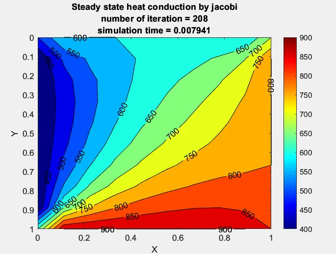
Jacobi Method:
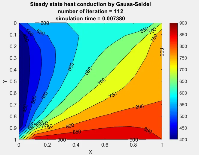
Gauss-seidel Method:
Successive Over Relaxation method:
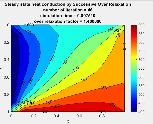
From the all above plots it can be inferred that the SOR method takes less time and less number of iterations when compare to the other two methods. Therefore SOR stands out to be good and fastest among all.
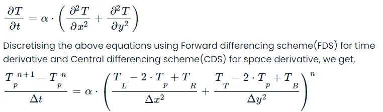
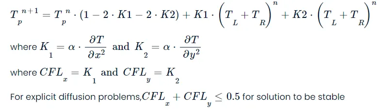
Unsteady State Analysis by both IMPLICIT and EXPLICIT Method:
IMPLICIT Method:

Jacobi method:

Gauss seidel method:

EXPLICIT Method:
Code for Unsteady State Analysis by IMPLICIT Method
% Unsteady state heat conduction with IMPLICIT Method

clear all
close all
clc

%initial conditions
%L = 1
nx = 10;
ny = 10;
nt = 300;
x = linspace(0,1,nx);
y = linspace(0,1,ny);
dx = x(2) - x(1);
dy = y(2) - y(1);


% Boundary condition

t = 300*ones(nx,ny);
t(:,1) = 400;
t(1,:) = 600;
t(:,ny) = 800;
t(nx,:) = 900;

% defining the temperature at corner points

t(1,1) = 500;
t(nx,ny) = 850;
t(1,ny) = 700;
t(nx,1) = 650;

dt = 0.01; %time step
told=t;
alpha = 0.3; % Thermal diffusivity
tprev_dt = told;

tol = 1e-4;
k1 = alpha*dt/(dx^2);
k2 = alpha*dt/(dy^2);

method = input('Iterative method = ');

%JACOBI ITERATIVE METHOD

if (method==1)
    tic;
    jacobi = 1;
    for p = 1:nt
        error =100;
         while(error>tol)
        for i = 2:(nx-1)
            for j = 2:(ny-1)
                term1 = (1+(2*k1)+(2*k2))^-1;
                term2 = k1*term1;
                term3 = k2*term1;
                h = (told(i-1,j)+told(i+1,j));
                v = (told(i,j+1)+told(i,j-1));
                t(i,j) = ((tprev_dt(i,j)*term1)+(h*term2)+(v*term3));
            end
        end

    error = max(max(abs(t-told)));
    told = t;
    jacobi = jacobi+1;
         end
         tprev_dt = t ;
    end
    time_taken = toc;

%plotting
figure(1)
contourf(x,y,t,'ShowText','on');
colormap(jet);
colorbar;
set(gca,'ydir','reverse')
xlabel('X')
ylabel('Y')
text1 = sprintf('number of iteration = %d', jacobi);
text2 = sprintf('simulation time = %f', time_taken);
title({'Unsteady state heat conduction with Implicit by Jacobi '; text1; text2});
end


%GAUSS-SEIDEL ITERATIVE METHOD

if (method==2)
    tic;
    gauss = 1;
    for p = 1:nt
        error =100;
         while(error>tol)
        for i = 2:(nx-1)
            for j = 2:(ny-1)
                term1 = (1+(2*k1)+(2*k2))^-1;
                term2 = k1*term1;
                term3 = k2*term1;
                h = (t(i-1,j)+told(i+1,j));
                v = (told(i,j+1)+t(i,j-1));
                t(i,j) = ((tprev_dt(i,j)*term1)+(h*term2)+(v*term3));
            end
        end

    error = max(max(abs(t-told)));
    told = t;
    gauss = gauss+1;
         end
         tprev_dt = t;
    end
    time_taken = toc;

%plotting
figure(1)
contourf(x,y,t,'ShowText','on');
colormap(jet);
colorbar;
set(gca,'ydir','reverse')
xlabel('X')
ylabel('Y')
text1 = sprintf('number of iteration = %d', gauss);
text2 = sprintf('simulation time = %f', time_taken);
title({'Unsteady state heat conduction with Implicit by Gauss-seidel'; text1; text2});
end

%SUCCESSIVE OVER RELAXATION ITERATIVE METHOD

if (method==3)
    tic;
    sor = 1;
    omega = 1.2; % Over relaxation factor
    for p = 1:nt
        error =100;
         while(error>tol)
        for i = 2:(nx-1)
            for j = 2:(ny-1)
                term1 = (1+(2*k1)+(2*k2))^-1;
                term2 = k1*term1;
                term3 = k2*term1;
                h = (t(i-1,j)+told(i+1,j));
                v = (told(i,j+1)+t(i,j-1));
                t(i,j) = (told(i,j)*(1-omega))+(omega*((tprev_dt(i,j)*term1)+(h*term2)+(v*term3)));
            end
        end

    error = max(max(abs(t-told)));
    told = t;
    sor = sor+1;
         end
         tprev_dt = t ;
    end
    time_taken = toc;

%plotting
figure(1)
contourf(x,y,t,'ShowText','on');
colormap(jet);
colorbar;
set(gca,'ydir','reverse')
xlabel('X')
ylabel('Y')
text1 = sprintf('number of iteration = %d', sor);
text2 = sprintf('simulation time = %f', time_taken);
title({'Unsteady state heat conduction with Implicit by Successive Over Relaxation'; text1; text2});
end
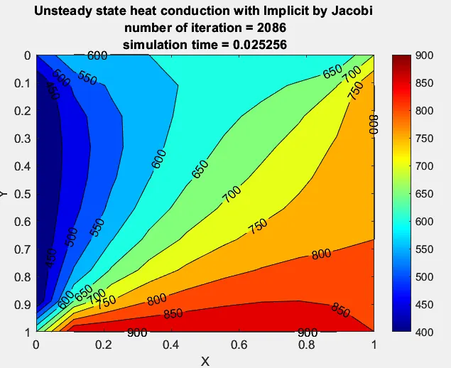
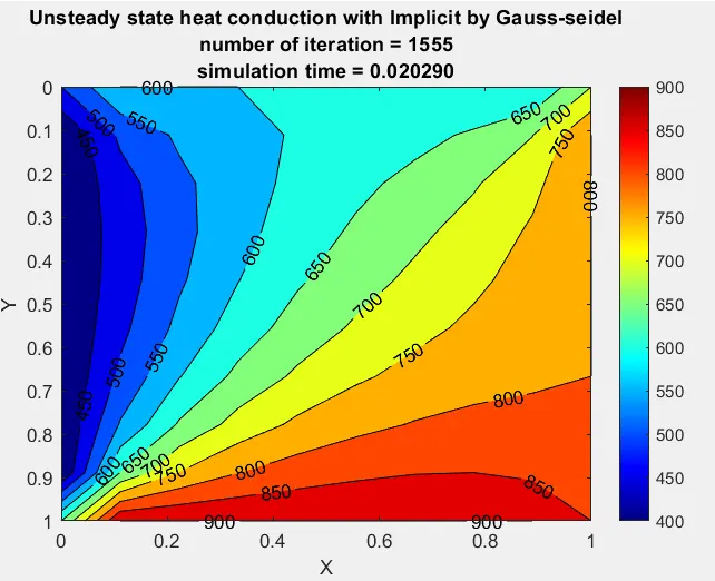
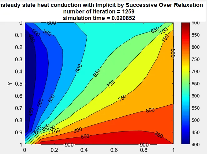
GRAPH:
Jacobi Method:
Gauss-seidel Method:
Successive Over Relaxation method:
Code for Unsteady State Analysis by EXPLICIT Method
% Unsteady state heat conduction with EXPLICIT


%initial conditions
%L = 1
nx = 10;
ny = 10;
nt = 300; % No.of steps
x = linspace(0,1,nx);
y = linspace(0,1,ny);
dx = x(2) - x(1);
dy = y(2) - y(1);

% initial temp condition

t = 300*ones(nx,ny);
t(:,1) = 400;
t(1,:) = 600;
t(:,ny) = 800;
t(nx,:) = 900;

% defining the temperature at corner points

t(1,1) = 500;
t(nx,ny) = 850;
t(1,ny) = 700;
t(nx,1) = 650;

dt = 0.01; %time step
told=t;
alpha = 0.3; % Thermal diffusivity

k1 = (alpha*dt)/(dx^2);
k2 = (alpha*dt)/(dy^2);
CFL = alpha*dt/(dx^2);

%EXPLICIT METHOD
% running for loop

tic;
    explicit = 1;
    for p = 1:nt
        for i = 2:(nx-1)
            for j = 2:(ny-1)
                term1 = (told(i-1,j)-2*told(i,j)+told(i+1,j));
                term2 = (told(i,j-1)-2*told(i,j)+told(i,j+1));
                t(i,j) = ((told(i,j))+(k1*term1)+(k2*term2));
            end
        end

    told = t;
    explicit = explicit+1;
    end

  time_taken = toc;

 %Plotting
figure(1)
contourf(x,y,t,'ShowText','on');
colormap(jet);
colorbar;
set(gca,'ydir','reverse')
xlabel('X')
ylabel('Y')
text1 = sprintf('timetaken = %d', dt*nt);
text2 = sprintf('simulation time = %f', time_taken);
title({'Unsteady state heat conduction with Explicit'; text1; text2});
GRAPH:
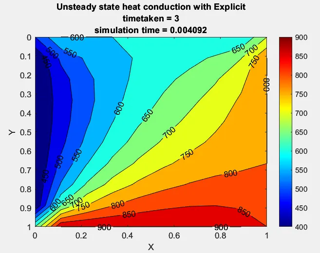
From above simulation we can see explicit method is converging faster than implicit methods taking less time for simulations
| S.no | Method | No. of iterations |
| 1. | Steady state (Jacobi) | 208 |
| 2. | Steady state (Gauss seidel) | 112 |
| 3. | Steady state (Successive over relaxation) | 46 |
| 4. | Unsteady state (Implicit Method, Jacobi) | 2086 |
| 5. | Unsteady state (Implicit Method, Gauss seidel) | 1555 |
| 6. | Unsteady state (Implicit Method, Successive over relaxation) | 1259 |
| 7. | Unsteady state (Explicit Method) | - |
From the table, For both steady and unsteady state we can clearly see that the Jacobi method takes lot of iterations to converge and successive over relaxation method takes the least
Order of method based on iterations,
Jacobi>Gauss seidel>Successive over relaxation
CONCLUSION:
- The 2D heat conduction equation is solved by using the point iterative techniques using the methods like Jacobi, Gauss-seidel, Successive over-relaxation for both implicit and explicit schemes.
- The temperature distribution plots are plotted for each methods.
- The number of iterations for each methods are calculated and displayed in the above table.