Week 7 - Simulation of a 1D Supersonic nozzle flow simulation using Macormack Method
AIM:
To simulate the isentropic flow through a quasi 1D subsonic-supersonic nozzle. By deriving both the conservation and non-conservation forms of the governing equations and sovle them using the MacCormack's technique. we need to determine the steady-state temperature distribution for the flow-field variables and investigate the difference between the two forms of governing equations by comparing their solutions.
OBJECTIVE:
To determine the steady-state temperature distribution for the flow-field variables and investigate the difference between the two forms of governing equations by comparing their solutions.
We need to show the following plots inside your report
1. Steady-state distribution of primitive variables inside the nozzle
2. Time-wise variation of the primitive variables
3. Variation of Mass flow rate distribution inside the nozzle at different time steps during the time-marching process
4. Comparison of Normalized mass flow rate distributions of both forms
PROCEDURE:
Consider a steady state isentropic flow through a convergent-divergent nozzle
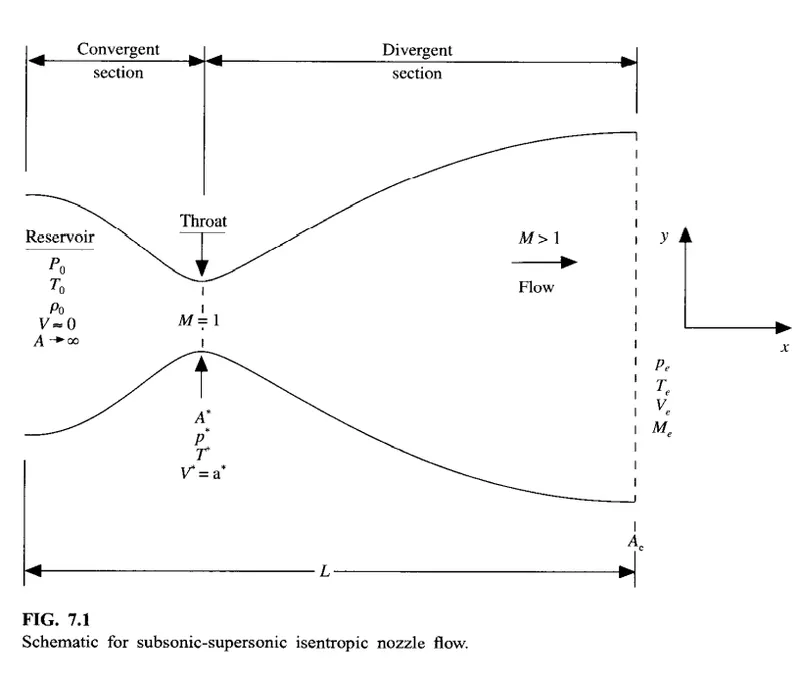
Here the flow at the inlet to the nozzle comes from the reservior where the pressure and temperature is denoted by po and To . The cross setional area is very large so (A->infinity) .The velocity is very small (V->0)
The governing continuity, momentum,and energy equation for this quasi-one-dimensional,steady,isentropic flow can be expressed as
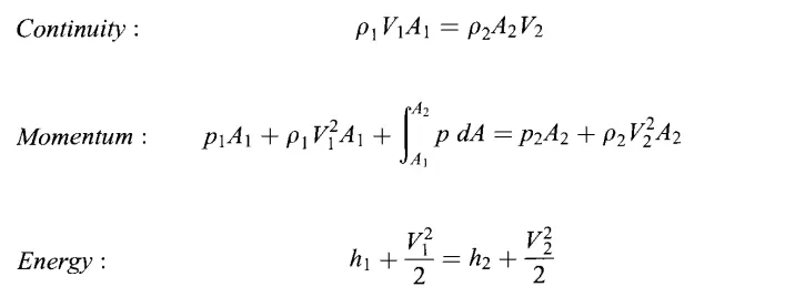
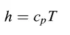
Where h = prefect gas,
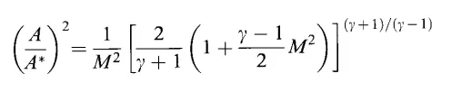
The Mach number variation through the nozzle is calculated by

To simulate the flow we need to do the following steps
1.Meshing is the process of divinding a continuous geometry into discrete geometric cells. Each cell is seperated by a node.
2. Discretisation is the process of converting the above PDEs into algebraic equations
3. Solving the discretised PDEs. Based on the type of PDEs different methods are chosen. The type of PDE in our case is hyperbolic so we are using the Mac Cormac method
MacCormac Method
It is an explicit finite difference technique which is second order accurate for both space and time. It is easy to work with and the solutions obtained are stable. The procedure is as follows
1. Predictor step:
Here we use the numerical method to calculate the required derivatives using the forward differencing scheme.
2. Solution update:
We will add the change obtained from the above predictor step to the original variable.
3. Primitive Variables:
For the conservative form we calculate the primitive variables from the solution vectors, flux vectors and source terms.
4. Corrector Step:
We use the numerical method to calculate the same derivatives we calculated in the first step again using the backward differencing scheme.
5. Calculating the average:
We take the average of derivatives we obtained in step 1 and step 4.
6. Final solution update:
We add the final change we calculated in step 5 to the original variable. This would be the final answer.
To simulate the supersonic flow we solve the flow equations of both the forms
GOVERNING EQUATION FOR NON CONSERVATIVE FORM:
Continuity Equation:

Momentum Equation:

Energy Equation:

Initial & Boundary Condition :
Initial condition:
The nozzle shape, A = A(x), is specified and held fixed, independent of time, For the case illustrated in this section, we choose a parabolic area distribution given by

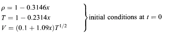
For Density, Temperature and Velocity is given by
Boundary condition:
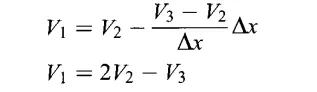
Inflow Boundary Condition:
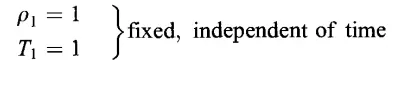
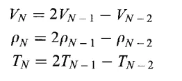
Outflow Boundary Condition:
GOVERNING EQUATION FOR CONSERVATIVE FORM:
Continuity Equation:
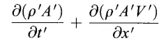
Momentum Equation:

Energy Equation:

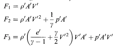
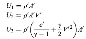
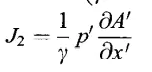
We cant use the above equations to write as code in MATLAB, So we change the above equation into Source term (J) ,Flux term(F) and solutions vector (U)
(i) FLUX TERMS:
(ii) SOLUTIONS VECTOR:
(iii) SOURCE TERM:
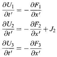
with these terms we can rewrite the governing equation of conservative form:
Initial & Boundary Condition :
Initial condition:
The nozzle shape, A = A(x), is specified and held fixed, independent of time, For the case illustrated in this section, we choose a parabolic area distribution given by
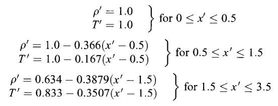
Density and Temperature for U1,U2,U3:
Boundary condition:
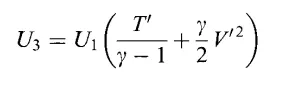
Inflow Boundary Condition:


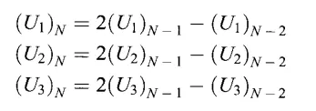
Outflow Boundary Condition:
Referred book for derivation and equations: CFD Basics by John D Anderson
MATLAB CODE:
close all
clear all
clc

%length of nozzle
L=3;
%number of grid points
n=[31 61];
%number of time steps
nt=1:1400;
%CFL number
cfl = 0.5;

for i = 1:length(n)
x=linspace(0,L,n(i));
[mfr_nc,mfr_throat_nc]=non_conservative(L,n(i),nt,cfl);
[mfr_c,mfr_throat_c]=conservative(L,n(i),nt,cfl);

figure(7)
subplot(2,1,1)
plot(nt,mfr_throat_c,'b',nt,mfr_throat_nc,'r','linewidth',1)
xlabel('Time steps (nt)')
ylabel('Mass flow rate')
legend('Conservative form','Non-Conservative form')
title('Mass flow rate"(Non-Conservative vs Conservative)" at throat point ')
grid on
subplot (2,1,2)
plot(x,mfr_c,'b',x,mfr_nc,'r','linewidth',1)
xlabel('Length of nozzle')
ylabel('Mass flow rate')
legend('Conservative form','Non-Conservative form')
title('Mass flow rate"(Non-Conservative vs Conservative)" in the nozzle')
grid on

figure(8)
subplot (2,1,1)
plot(nt,mfr_throat_c,'linewidth',1)
hold on
xlabel('Time steps (nt)')
ylabel('Mass flow rate')
legend('31st node','61st node')
title('Grid independency test at throat point(Conservative)')
grid on
subplot (2,1,2)
plot(nt,mfr_throat_nc,'linewidth',1)
hold on
xlabel('Time steps (nt)')
ylabel('Mass flow rate')
legend('31st node','61st node')
title('Grid independency test at throat point(Non-Conservative)')
grid on

figure(9)
subplot (2,1,1)
plot(x,mfr_c,'linewidth',1)
hold on
xlabel('Length of nozzle')
ylabel('Mass flow rate')
legend('31st node','61st node')
title('Grid independency test at the nozzle(Conservative form)')
grid on
subplot (2,1,2)
plot(x,mfr_nc,'linewidth',1)
hold on
xlabel('Length of nozzle')
ylabel('Mass flow rate')
legend('31st node','61st node')
title('Grid independency test at the nozzle(Non-Conservative form)')
grid on

end
FUNCTION CODE FOR NON CONSERVATIVE FORM:
function [mfr_nc,mfr_throat_nc]=non_conservative(L,n,nt,cfl)


x=linspace(0,L,n);
dx=x(2)-x(1);

% initial conditions rho, a, v, T, mfr, M, p
rho = 1-0.3146*x;
T= 1-0.2314*x;
v=(0.1+1.09*x).*T.^0.5;
%area
a= 1+2.2*(x-1.5).^2;
M= v./(T.^0.5);
mfr = rho.*a.*v;
p=rho.*T;
g = 1.4;%gamma value

for z=1:31
    u=(T(z))^(1/2);
    dt(z) = cfl*dx/(u + v(z));
end
dt=min(dt);

for i = 1:length(nt)
  %storing initial values
    rho_old = rho;
    T_old = T;
    v_old = v;
  for j=2:n-1
  %predictor step
    drho_dx = (rho(j+1)-rho(j))/dx;
    dv_dx = (v(j+1)-v(j))/dx;
    dT_dx = (T(j+1)-T(j))/dx;
    da_dx = (log(a(j+1))-log(a(j)))/dx;
     % continuity equation
    drho_dt_p(j) = -rho(j)*dv_dx - rho(j)*v(j)*da_dx - v(j)*drho_dx;
    % momentum equation
    dv_dt_p(j) = -v(j)*dv_dx - (1/g)*(dT_dx + (T(j)/rho(j))*drho_dx);
     % energy equation
    dT_dt_p(j) = -v(j)*dT_dx - (g-1)*T(j)*(dv_dx + v(j)*da_dx);
     %updating primitives
    v(j) = v_old(j) + dv_dt_p(j)*dt;
    rho(j) = rho_old(j) + drho_dt_p(j)*dt;
    T(j) = T_old(j) + dT_dt_p(j)*dt;
  %corrector step
    drho_dx = (rho(j)-rho(j-1))/dx;
    dv_dx = (v(j)-v(j-1))/dx;
    dT_dx = (T(j)-T(j-1))/dx;
    da_dx = (log(a(j))-log(a(j-1)))/dx;
     % continuity equation
    drho_dt_c(j) = -rho(j)*dv_dx - rho(j)*v(j)*da_dx - v(j)*drho_dx;
    % momentum equation
    dv_dt_c(j) = -v(j)*dv_dx - (1/g)*(dT_dx + (T(j)/rho(j))*drho_dx);
    % energy equation
    dT_dt_c(j) = -v(j)*dT_dx - (g-1)*T(j)*(dv_dx + v(j)*da_dx);
  end
  %average time derivatives
    drho_dt_avg = 0.5*(drho_dt_p + drho_dt_c);
    dv_dt_avg = 0.5*(dv_dt_p + dv_dt_c);
    dT_dt_avg = 0.5*(dT_dt_p + dT_dt_c);
  %final corected values
  for k = 2:n-1
    rho(k) = rho_old(k) + drho_dt_avg(k)*dt;
    v(k) = v_old(k) + dv_dt_avg(k)*dt;
    T(k) = T_old(k) + dT_dt_avg(k)*dt;
  end
  %entry boundary conditions
    v(1) = 2*v(2)-v(3);
  %exit boundary conditions
    v(n) = 2*v(n-1)-v(n-2);
    rho(n) = 2*rho(n-1)-rho(n-2);
    T(n) = 2*T(n-1)-T(n-2);
  %Final update of primitives
    p = rho.*T;
    M= v./T.^0.5;
    error(k) =  abs(v(k)-v(k-1));
    mfr= rho.*a.*v;
  %to find values at throat point
    T_throat(i) = T(16);
    rho_throat(i) = rho(16);
    v_throat(i) = v(16);
    M_throat(i) = M(16);
    p_throat(i) = p(16);
    error_throat(i)=error(16);
    mfr_throat(i)=mfr(16);
    if n==31
for ii=[1:50:201 700]
    if ii==i
       figure(1)
     plot(x,mfr,'linewidth',1)
     hold on
     title ('Mass flow rate inside the nozzle at different time steps(Non-Conservative)')
     xlabel('Length of nozzle')
     ylabel('Mass flow rate')
    elseif i==1400
     plot(x,mfr,'*r')
     legend('1','50','100','250','600','800','1400')
     grid on
    end
end
end

end
if n==31
figure(2)
     plot(x,v,'b',x,p,'r',x,T,'k',x,rho,'m',x,M,'g',x,mfr,'c')
     ylim([-0.1 3.7])
     title (sprintf('Time step = %d',i))
     xlabel('Length of nozzle')
     ylabel('Non dimensional parameters')
     legend('Velocity','Pressure','Temperature','Density','Mach number','Mass flow rate','location','northwest')
     title('Steady-state distribution of primitive variables inside the nozzle(Non-Conservative)')
     grid on

figure (3)
plot(nt,rho_throat)
hold on
plot(nt,v_throat,'linewidth',1)
plot(nt,p_throat,'linewidth',1)
plot(nt,T_throat,'linewidth',1)
plot(nt,M_throat,'linewidth',1)
plot(nt,mfr_throat,'linewidth',1)
xlabel('Time steps (nt)')
ylabel('Non dimensional parameters')
legend('Density','Velocity','Pressure','Temperature','Mach number','Mass flow rate')
title('Time-wise variation of the primitive variables at throat point(Non-Conservative)')
grid on
end
mfr_nc=mfr;
mfr_throat_nc=mfr_throat;
end
FUNCTION CODE FOR CONSERVATIVE FORM:
function [mfr_c,mfr_throat_c]=conservative(L,n,nt,cfl)

x=linspace(0,L,n);
dx=x(2)-x(1);

% initial conditions rho, a, v, T, M, mfr, p
for ii=1:length(x)
    if (x(ii)<=0.5)
        rho(ii) = 1;
        T(ii) = 1;
    elseif (x(ii)>0.5) & (x(ii)<=1.5)
        rho(ii) = 1-0.366*(x(ii)-0.5);
        T(ii)= 1-0.167*(x(ii)-0.5);
    elseif (x(ii)>1.5) & (x(ii)<=3.5)
        rho(ii) = 0.634-0.3879*(x(ii)-1.5);
        T(ii)= 0.833-0.3507*(x(ii)-1.5);
    end
end
a= 1+2.2*(x-1.5).^2;     %area
g = 1.4;                 %gamma value
% solution vectors u1, u2, u3
u1 = rho.*a;
u2 = 0.59*ones(1,n);
v=u2./u1;
u3 = u1.*((T./(g-1))+(g/2).*v.^2);

M= v./(T.^0.5);
mfr = rho.*a.*v;         %mass flow rate
p=rho.*T;                %pressure


for z=1:31
u=(T(z))^(1/2);
dt(z) = cfl*dx/(u + v(z));
end
dt=min(dt);

for i = 1:length(nt)
    %storing initial values
    u1_old = u1;
    u2_old = u2;
    u3_old = u3;

    for j=2:n-1
   %flux vectors
        f1 = u2;
        f2 = ((u2.^2)./u1)+((g-1)/g)*(u3-((g/2)*(u2.^2)./u1));
        f3 = ((g.*u2.*u3)./u1) - ((g*(g-1)/2)*(u2.^3)./(u1.^2));
   %source term
        j1 = (1/g)*rho(j)*T(j)*((a(j+1)-a(j))/dx);
   %predictor step
   %continuity equation
        du1_dt_p(j)= -(f1(j+1)-f1(j))/dx;
   %momentum equation
        du2_dt_p(j)= -(f2(j+1)-f2(j))/dx + j1;
   %energy equation
        du3_dt_p(j)= -(f3(j+1)-f3(j))/dx;
   %updating solution vectors
        u1(j) = u1_old(j) + du1_dt_p(j)*dt;
        u2(j) = u2_old(j) + du2_dt_p(j)*dt;
        u3(j) = u3_old(j) + du3_dt_p(j)*dt;
   %updating primitives
        rho=u1./a;
        T=(g-1).*(u3./u1-(g/2).*(u2./u1).^2);
   %updating flux terms
        f1=u2;
        f2=u2.^2./u1+((g-1)/g).*(u3-(g/2)*u2.^2./u1);
        f3=g.*u2.*u3./u1-0.5*g*(g-1).*u2.^3./u1.^2;
   %source term for corrector step
        j2 = (1/g)*(rho(j)*T(j)*(a(j)-a(j-1))/dx);
   %corrector step
   %continuity equation
        du1_dt_c(j) = -(f1(j)-f1(j-1))/dx;
   %momentum equation
        du2_dt_c(j) = -(f2(j)-f2(j-1))/dx + j2;
   %energy equation
        du3_dt_c(j) = -(f3(j)-f3(j-1))/dx;
    end
    %average time derivatives
        du1_dt_avg = 0.5*(du1_dt_p + du1_dt_c);
        du2_dt_avg = 0.5*(du2_dt_p + du2_dt_c);
        du3_dt_avg = 0.5*(du3_dt_p + du3_dt_c);
    %final corected values
    for k = 2:n-1
        u1(k) = u1_old(k) + du1_dt_avg(k)*dt;
        u2(k) = u2_old(k) + du2_dt_avg(k)*dt;
        u3(k) = u3_old(k) + du3_dt_avg(k)*dt;
    end
    %entry boundary conditions
        u1(1) = a(1);
        u2(1) = 2*u2(2)-u2(3);
        u3(1) = u1(1)*(T(1)/(g-1) + (g*(u2(1)/u1(1))^2)/2);
    %exit boundary conditions
        u1(n) = 2*u1(n-1)-u1(n-2);
        u2(n) = 2*u2(n-1)-u2(n-2);
        u3(n) = 2*u3(n-1)-u3(n-2);

    %Final update of primitives
        rho = u1./a;
        v = u2./u1;
        T=(g-1).*(u3./u1-(g/2).*(u2./u1).^2);
        p = rho.*T;
        M= v./T.^0.5;
        error(k) =  abs(v(k)-v(k-1));
        mfr= u2;
  %to find values at throat point
    T_throat(i) = T(16);
    rho_throat(i) = rho(16);
    v_throat(i) = v(16);
    M_throat(i) = M(16);
    p_throat(i) = p(16);
    error_throat(i)=error(16);
    mfr_throat(i)=mfr(16);

if n==31
    for ii=[1:50:201 700]
    if ii==i
       figure(4)
     plot(x,mfr,'linewidth',1)
     hold on
     title ('Mass flow rate distribution inside the nozzle at different time steps(Conservative) ')
     xlabel('Length of nozzle')
     ylabel('Mass flow rate')
    elseif i==1400
     plot(x,mfr,'*r')
     legend('1','50','100','250','600','800','1400')
     grid on
    end
end
end

end
if n==31
figure(5)
     plot(x,v,'b',x,p,'r',x,T,'k',x,rho,'m',x,M,'g',x,mfr,'c')
     ylim([-0.1 3.7])
     title (sprintf('Time step = %d',i))
     xlabel('Length of nozzle')
     ylabel('Non dimensional parameters')
     legend('Velocity','Pressure','Temperature','Density','Mach number','Mass flow rate','location','northwest')
     title('Steady-state distribution of primitive variables inside the nozzle(Conservative)')
     grid on

figure (6)
plot(nt,rho_throat)
hold on
plot(nt,v_throat,'linewidth',1)
plot(nt,p_throat,'linewidth',1)
plot(nt,T_throat,'linewidth',1)
plot(nt,M_throat,'linewidth',1)
plot(nt,mfr_throat,'linewidth',1)
xlabel('Time steps (nt)')
ylabel('Non dimensional parameters')
legend('Density','Velocity','Pressure','Temperature','Mach number','Mass flow rate')
title('Time-wise variation of the primitive variables at throat point (Conservative)')
grid on
end
mfr_c=mfr;
mfr_throat_c=mfr_throat;

end
RESULT GRAPHS:
Steady-state distribution of primitive variables inside the nozzle
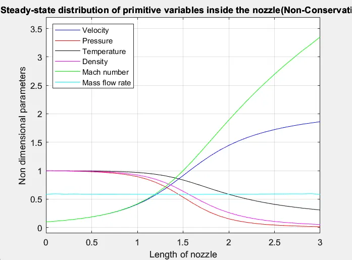
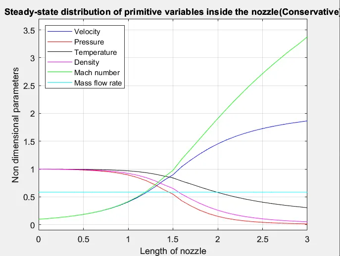
we can see from the above plot that the primitive variable such as Pressure, Density and Temperature decrease along the length of the nozzle as the Mach number and velocity increases along the length of the nozzle for both conservative and non conservative forms. Both gives almost similar solution
Time-wise variation of the primitive variables:
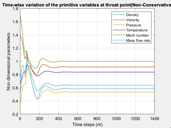
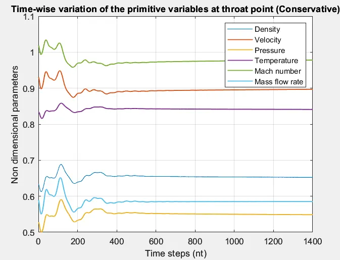
We can see from the above plot ,that in conservative form, the solution varies in small amounts with time step as compared to non-conservative form. The non-conservative equations give a wavy curve at beginning but as the time steps increase, it also becomes stable. After 600-700 time steps, the primitive variables are constant for any time step above 700-time steps throughout the nozzle. This conservation gives a steady state solution soon as compared to non-conservation.
Variation of Mass flow rate distribution inside the nozzle at different time steps during the time-marching process
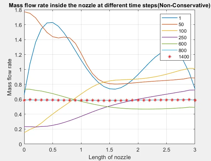
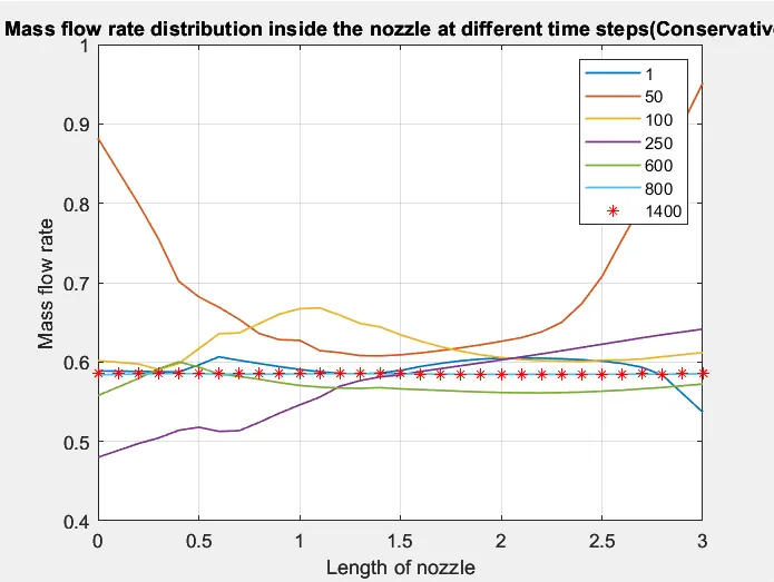
We can see from the above plot ,that Mass Flow Rate at different Time steps along the length of the nozzle fluctuates initially, however the solution becomes stable after the 600th Timestep for both the forms attaining a constant value.
Comparison of Normalized mass flow rate distributions of both forms
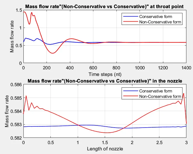
We can see form the above plot that the Non Conservative mass flow rate is deviating more than the conservative mass flow rate in result with respect to time step and length of the nozzle ,hence in a study about mass flow rate the conservative form is much more reliable than the non conservative form.
Grid Dependency test:
In order to conduct grid dependency test, here we are considering two grid points one is 31 grid points and other with 61 grid points and varying their massflow rate with both time steps as well as for length of the nozzle in both throat and nozzle area
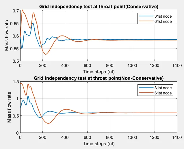
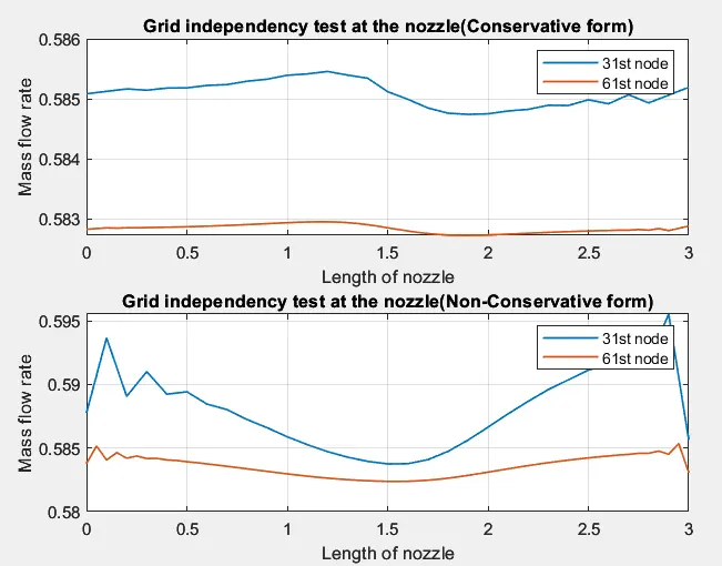
From the above table it can be seen that the increase in grid point will increase the accuracy but the run time of the simulation also drastically increase with the increase in the number of grid points. It means that faster result less is accuracy.
Considering all the results we can conclude that Conservative form converges slightly faster than Non Conservative form offering stable solution along the simulation. But we can take both the forms because both are dependable for calculating the equation which gives almost precise solution.
CONCLUSION:
- Simulated the isentropic flow through a quasi 1D subsonic-supersonic nozzle by deriving both the conservation and non-conservation forms of the governing equations and sovled them using the MacCormack's technique.
- Steady-state distribution of primitive variables inside the nozzle is calculated and plotted
- Time-wise variation of the primitive variables is calculated and plotted
- Variation of Mass flow rate distribution inside the nozzle at different time steps during the time-marching process is calculated and plotted
- Comparison of Normalized mass flow rate distributions of both forms is calculated and plotted