Week 4 - CHT Analysis on Exhaust port

AIM:
To run simulation to analyse Conjugate Heat transfer in Exhaust port.

1. Give a brief description of why and where a CHT analysis is used.
2. Maintain the y+ value according to the turbulence model and justify the results.
3. Calculate the wall/surface heat transfer coefficient on the internal solid surface & show the velocity & temperature contours in appropriate areas.
4. How would you verify if the HTC predictions from the simulations are right? On what factors does the accuracy of the prediction depend on?

PROCEDURE:

Conjugate Heat Transfer (CHT):

The Conjugate Heat Transfer (CHT) analysis type allows for the simulation of heat transfer between solid and fluid domains by exchanging thermal energy at the interfaces between them.

where a CHT analysis is used

Internal Combustion Engines

The Internal Combustion Engine industry is moving toward simulating the entire system rather than independent components. The accuracy of the predicted combustion in the cylinder is dependent on the temperature boundary conditions in the cylinder. By considering heat transfer in the metal components (e.g., the cylinder head, liner, piston, etc.), the cylinder wall no longer has a user-specified temperature, but instead has temperatures predicted as part of the complete-system simulation. This makes the overall simulation results more predictive by reducing the dependence on assumed boundary conditions.

Pumps and Compressor

Resolving the spatially varying surface temperature distributions in pumps and compressors improves the accuracy of the simulation and provides useful temperature data. For example, in a twin screw compressor, thermal expansion affects the clearance between the rotors. If that effect is not captured, the simulations will incorrectly predict leakage flows and lower the accuracy of your results.

SETUP:

Geometry:

• Load the CAD model of Exhaust manifold in Spaceclaim and check for any extra edges, remove them if any.
• Go to Repair -> Volume extract, and select the edges to separate inner and outer volume. Name the outer volume as Solid volume and inner ass Fluid volume and move bothe the volume to new component and delete empty components.
• Go to workbench -> Shareprep, to share the physics between the fluid and solid volume and conformal mesh can be achieved. pink coloured circle are seen after completing the process.
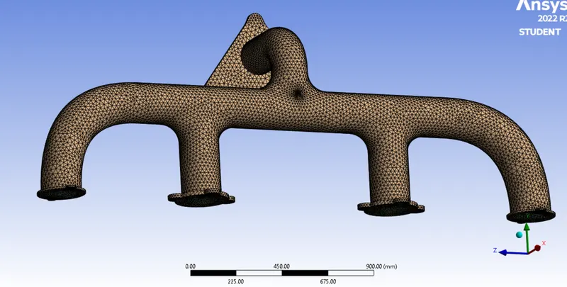
• The exhaust port is a three-dimensional model containing four inlets and one outlet. Despite having isothermal boundary conditions and a uniform flow rate at the four inlets, the model cannot be cut into two halves to save computational time because of its asymmetrical nature. Therefore the whole model is discretized and is considered for meshing.
• CHT analysis requires both the solid and the liquid volume under consideration, Spaceclaim gives an option of volume extract for selecting edges for fluid volume.
• Both the solid volume and liquid volume are copied into one component.
• Share topology is created.
• Spaceclaim gives an option for share coincident topology, when share coincident topology is selected and executed, the mesh from the fluid volume and the solid volume are said to be conformal with each other which is a requirement for CHT analysis.
• The exhaust port is loaded into the meshing window and then simulated for baseline mesh and the refined mesh.
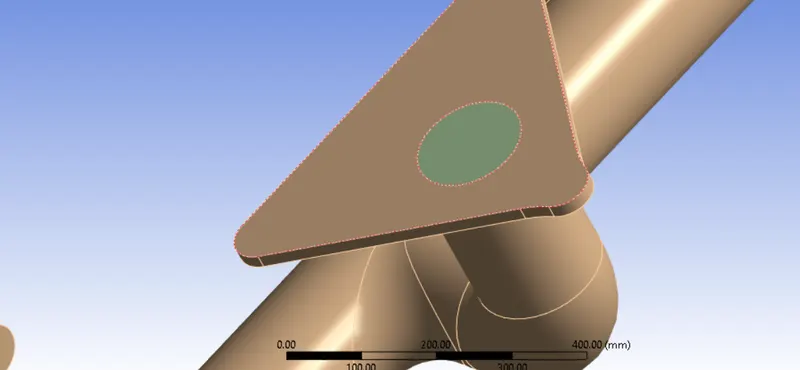
• The named selections are created ( inlet, outlet, outer wall convection)
• The necessary contour images and graphs are studied to understand the behavior of temperature, velocity, and surface heat transfer coefficient at the interface.

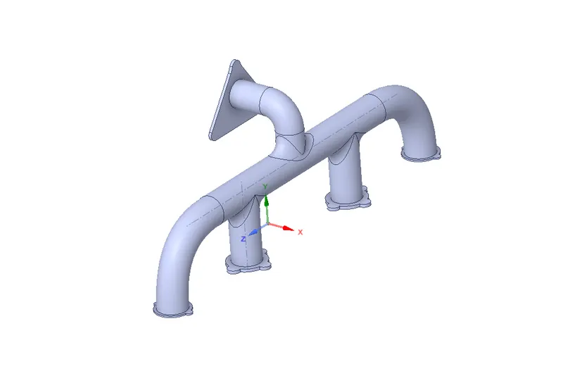
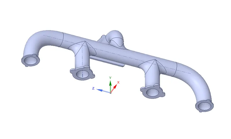
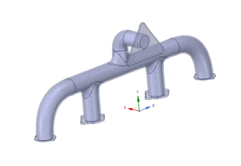
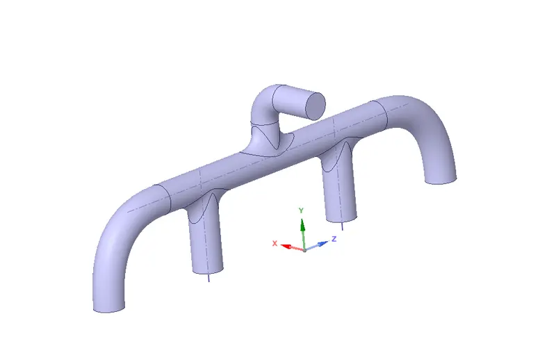
Meshing:

• It is the process of discretizing the geometry into a small number of volumes containing nodes.
• Since the geometry is complex and the mesh is unstructured therefore the finite volume scheme is used as a discretization scheme.
• Select the mesh and generate base mesh of default size as 100 mm.
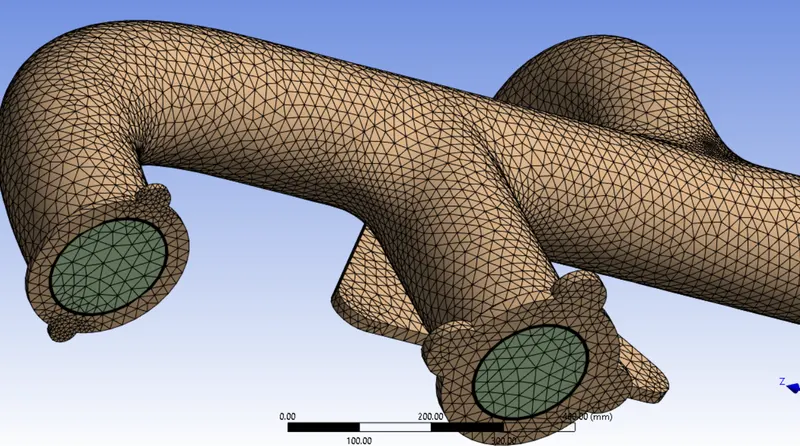
• Now hide the outer body and select the inner face and named it as inflation layer.Go to inflation layer and select inflation layer and maximum thickness of 5 mm.
• To refine the mesh size further, Go to mesh -> sizing and add mesh size of 50 mm.

Solver:

Solver: Presure based steady state solver.

Boundary Conditions:

Inlet

Velocity = 5 m/s

Temperature = 700 K.

Outlet:

Pressure = 0 Pa (Gauge pressure)

Outlet wall convection:

Thermal condition: Convection

Heat transfer coefficient = 20 W/m2K.

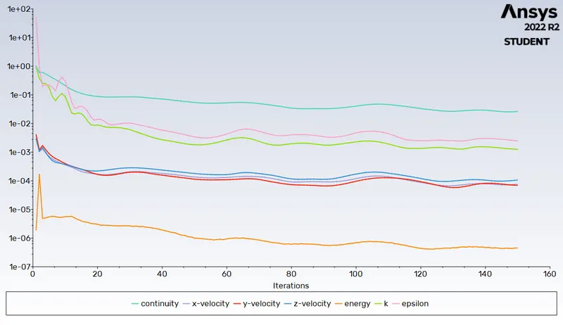
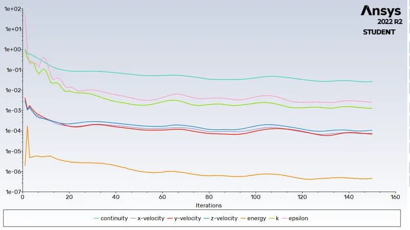
Residual Plot:

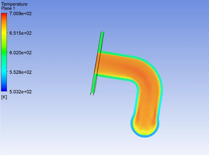
Temperature Contour:

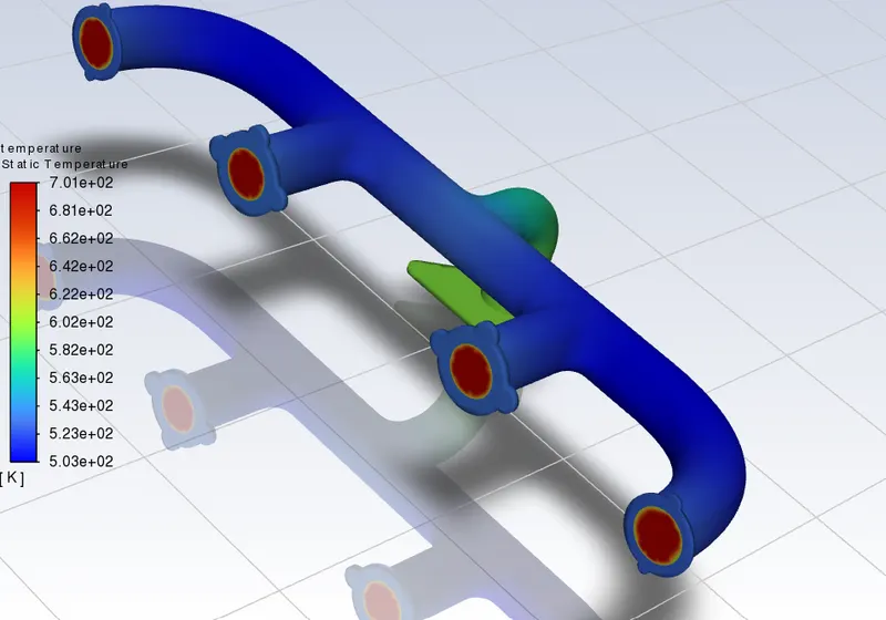
Temperature:

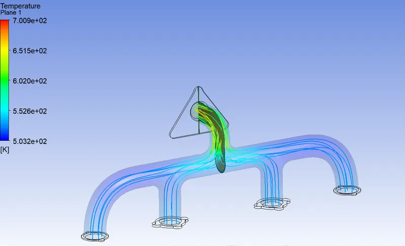
Temperature Steamlines:

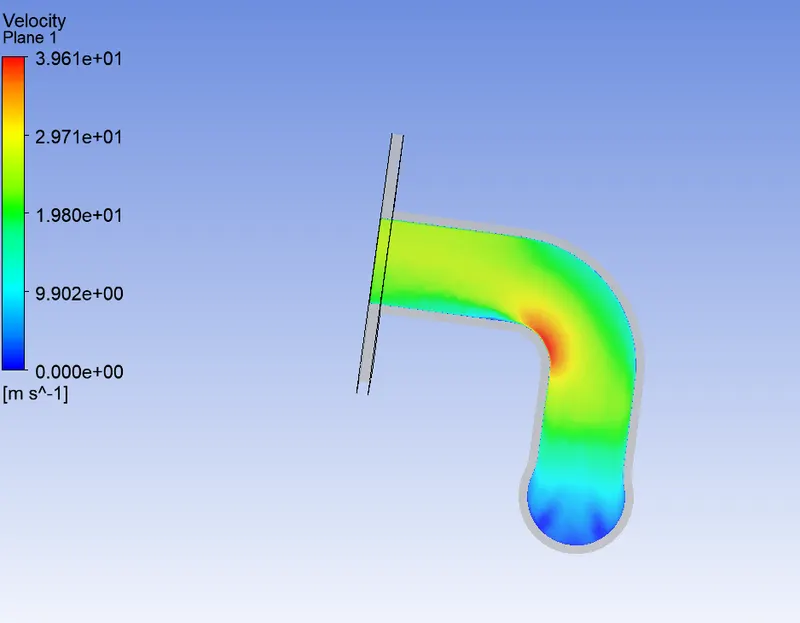
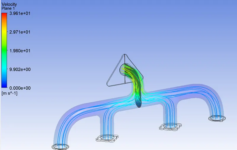
Velocity :

Velocity Steamlines:

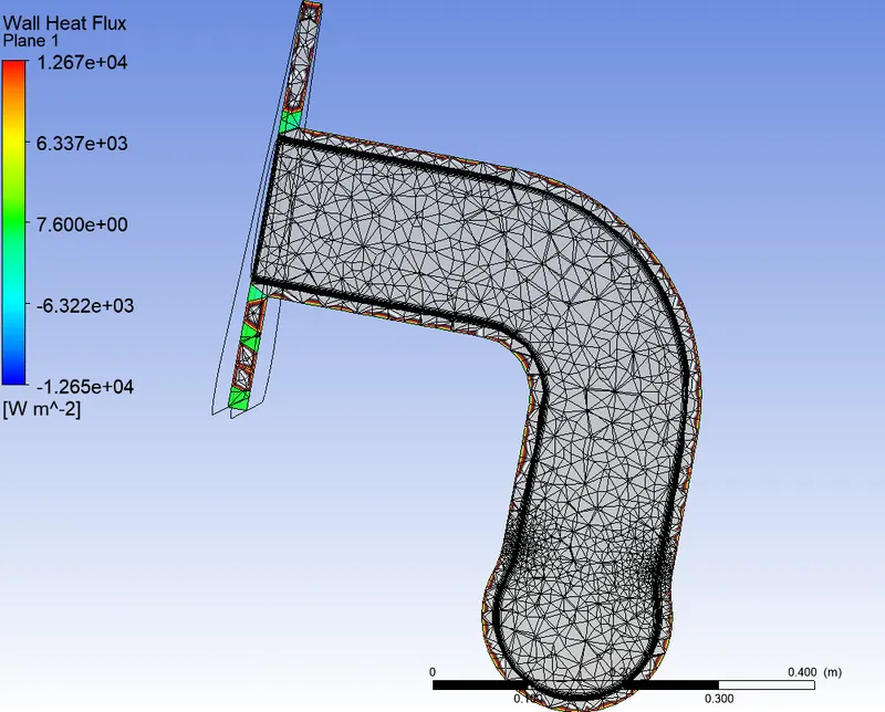
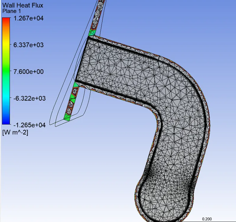
Wall heat flux:

Even more refined mesh is done with element size 110mm and sizing mesh size 60mm with inflation layer =8

Residual Plot:

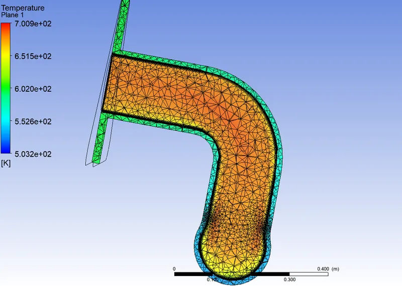
Temperature Contour:

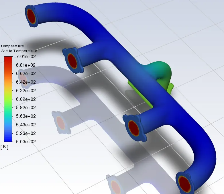
Temperature:

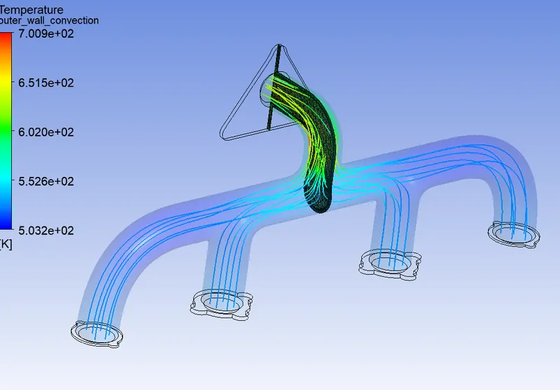
Temperature streamline:

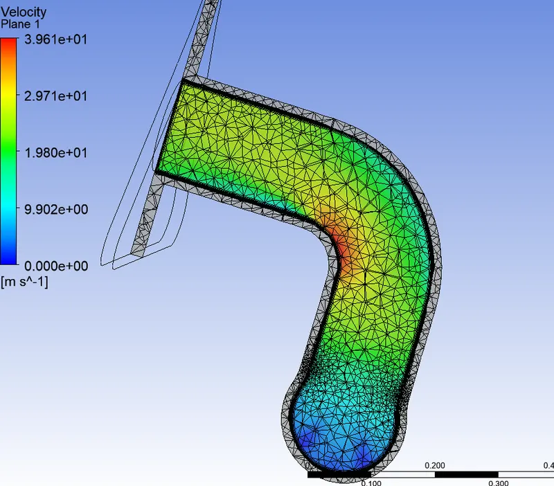
Velocity:

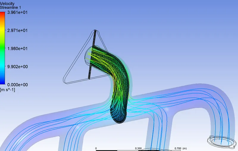
Velocity Steamlines:

Wall heat flux:

How would you verify if the HTC predictions from the simulations are right? On what factors does the accuracy of the prediction depend on?

The typical flow conditions in automotive exhaust systems produce are in the range of 10^3 to 5*10^4. The exhaust flow often enters the region re<2300, especially in exhaust manifold runners. In spite of that, the flow remains actually turbulent since it has flowed through a substantial restriction. The exhaust valves and the persisting unsteady flow pulsation effects don’t favor the transition to the laminar region.

According to the sieder tate relation which correlates the Nu number with Re and Pr

Nu = 0.027Re^0.8Pr^1/3

It means Nusselt no. is the function of Reynolds no and Prandtl number

As the turbulent boundary layer in the bend of the outlet port is the thin maximum velocity of flow is observed at bend and hence higher Reynolds number.

Now, Nu = h*L/k

As the length of pipe and thermal conductivity is a constant value of h will increase as Nu increases and Nu increases as Re increases.

As per our result, the heat transfer coefficient is high for a higher value of velocity and hence our results are correct.

Accuracy of HTC prediction :

Accuracy of the predictions depends on several things ,

• Accurate geometry of model.
• Mesh quality.
• Inflation layers
• Properties of material being used.
• Turbulence models.

RESULT:

• From the above both cases output, we can say that the results are almost same but the refined mesh gives us more smoothness and accuracy.
• Two factors influence the performance simultaneously: (a) Flow is developing along the length and the heat transfer coefficients tend to decrease along flow (b) Turbulence;
• At the same time, turbulence is developing with tube rows at bent, which would increase heat transfer coefficients.
• The maximum heat transfer results at bend of exit port, It is because to ensure conservation of mass at exit port velocity should more, which resuts in higher velocity and increse in velocity attain a Reynolds number that is sufficient to make flow trurbulent and higher Nusselt number at pipe bent at exit, which increses Heat transfer co-efficient at that location.