Challenge

Week 3.5 - Deriving 4th order approximation of a 2nd order derivative using Taylor Table method

HHemavarshini R V22 Feb 2023

AIM:

To Derive the 4th order approximations of the second-order derivative of a function for the following numerical schemes.

1. Central difference

2. Skewed right-sided difference

3. Skewed left-sided difference

OBJECTIVE:

After deriving these schemes, prove that your skewed schemes are fourth-order accurate i.e the thumb rule given in HINT (ii).
Once you have done this, write a program in Matlab to evaluate the second-order derivative of the analytical function exp(x)*cos(x) and compare it with the 3 numerical approximations that you have derived.
Provide a plot that compares the absolute error between the above-mentioned schemes
In your own words, describe why a skewed scheme is useful? What can a skewed scheme do that a CD scheme cannot?

PROCEDURE:

CENTRAL DIFFERENCING SCHEME:

Here the nodes selected are symmetrical i.e. the data is taken from both sides of point of focus. Using Taylor’s method, we get

∂^2f/∂x2=af(i-2)+bf(i-1)+cf(i)+df(i+1)+ef(i+2)

NOTE: - To select the number of nodes , we can use following expression:

N=p + q -1 (central differencing)

N = p + q (skewed differencing)

Here N = no. of nodes, p = order of derivative and q = order of approximation.

The number of nodes = p+q-1

The no of nodes = 2+4-1 =>5.

Taylor’s table for Central difference:

	f(X)	dx f’(x)	dx² f’’(x)	dx³f’’’(x)	dx⁴ f’’’’(x)	dx⁵ f’’’’’(x)
af(i-1)	a	-2a	4a/2	-8a/6	16a/24	-32a/120
bf(i-2)	b	-b	b/2	-b/6	b/24	-b/120
cf(i)	c	0	0	0	0	0
df(i-1)	d	d	d/2	d/6	d/24	d/120
ef(i-2)	e	2e	4e/2	8e/6	16e/24	32e/120
af(i-2) +bf(i-1) +cf(i) +df(i+1) + ef(i+2)	0	0	1	0	0	?

This table transform into matrix of type AX=B

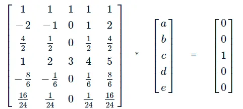on further solving we get the values of the unknown

i.e. Values = a = -0.0833

b= 1.3333

c= -2.5000

d= 1.3333

e= -0.0833

Skewed right sided difference:

When the data point of the left nodes are not available (at initial boundary conditions) then we have to rely on the available data set.

∂^2f/∂x^2=af(i)+bf(i+1)+cf(i+2)+df(i+3)+ef(i+4)+ff(i+5)

The number of nodes = p+q

The no of nodes = 2+4 =>6.

Taylor’s table for Skewed right sided difference:

	f(x)	dx f’ (X)	dx² f’’ (x)	dx³ f’’’(x)	dx⁴f’’’’(x)	dx⁵f’’’’’(x)
af(i)	a	0	0	0	0	0
bf(i+1)	b	b	b/2	b/6	b/24	b/120
cf(i+2)	c	2c	4c/2	8c/6	16c/24	32c/120
df(i+3)	d	3d	9d/2	27d/6	81d/24	243d/120
ef(i+4)	e	4e	16e/2	64e/6	256e/24	1024e/120
ff(i+5)	f	5f	25f/2	125f/6	625f/24	3125f/120
af(i) + bf(i+1) + cf(i+2) + df(i+3) + ef(i+4) +ff(i+5)	0	0	1	0	0	0

This table transform into matrix of type AX=B

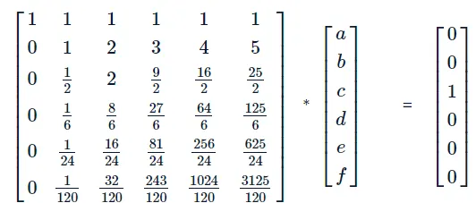on further solving we get the values of the

unknown

i.e. Values =

a = 3.7500

b= -12.8333

c= 17.8333

d= -13.0000

e= 5.0833

f= -0.8333

Skewed left sided difference: -

When the data point of the right nodes are not available (at boundary conditions) then we have to rely on the available data set.

∂^2f/∂x^2=af(i-5)+bf(i-4)+cf(i-3)+df(i-2)+ef(i-1)+ff(i)

Taylor’s table for Skewed left sided difference:

	f(x)	dx f’ (X)	dx² f’’ (x)	dx³ f’’’(x)	dx⁴f’’’’(x)	dx⁵f’’’’’(x)
af(i-5)	a	-5a	25a/2	-125a/6	625a/24	-3125a/120
bf(i-4)	b	-4b	16b/2	-64b/6	256b/24	-1024b/120
cf(i-3)	c	-3c	9c/2	-27c/6	81c/24	-243c/120
df(i-2)	d	-2d	4d/2	-8d/6	16d/24	-32d/120
ef(i-1)	e	-e	e/2	-e/6	e/24	-e/120
ff(i)	f	0	0	0	0	0
af(i-5) + bf(i-4) + cf(i-3) + df(i-2) + ef(i-1) +ff(i)	0	0	1	0	0	0

This table transform into matrix of type AX=B:

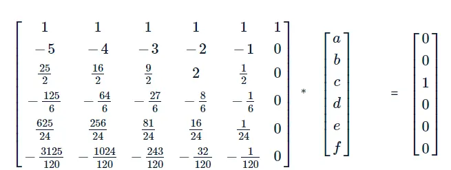on further solving we get the values of the unknown

i.e. Values = a = -0.8333

b= 5.0833

c=13.0000

d= 17.8333

e= -12.8333

f= 3.7500

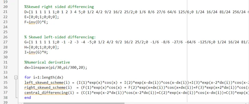
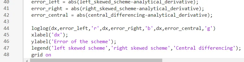
MATLAB CODE:

clear all

close all

clc

% analytical derivative

%f(x)=exp(x)cosx

%f'(x)= exp(x)cosx-exp(x)sinx

%f''(x)=-2exp(x)sinx

%inputs

x= pi/5;

analytical_derivative = -2*exp(x)*sin(x);

% Central differencing

A=[1 1 1 1 1;-2 -1 0 1 2; 2 1/2 0 1/2 2;-8/6 -1/6 0 1/6 8/6;16/24 1/24 0 1/24 16/24];

B=[0;0;1;0;0];

C=inv(A)*B;

%Skewed right sided differencing

D=[1 1 1 1 1 1;0 1 2 3 4 5;0 1/2 4/2 9/2 16/2 25/2;0 1/6 8/6 27/6 64/6 125/6;0 1/24 16/24 81/24 256/24 625/24;0 1/120 32/120 243/120 1024/120 3125/120];

E=[0;0;1;0;0;0];

F=inv(D)*E;

% Skewed left-sided differencing:

G=[1 1 1 1 1 1;0 -1 -2 -3 -4 -5;0 1/2 4/2 9/2 16/2 25/2;0 -1/6 -8/6 -27/6 -64/6 -125/6;0 1/24 16/24 81/24 256/24 625/24;0 -1/120 -32/120 -243/120 -1024/120 -3125/120];

H=[0;0;1;0;0;0];

I=inv(G)*H;

%Numerical derivative

dx=linspace(pi/30,pi/300,20);

for i=1:length(dx)

left_skewed_scheme(i) = (I(1)*exp(x)*cos(x) + I(2)*exp(x-dx(i))*cos(x-dx(i))+I(3)*exp(x-2*dx(i))*cos(x-2*dx(i))+I(4)*exp(x-3*dx(i))*cos(x-3*dx(i))+I(5)*exp(x-4*dx(i))*cos(x-4*dx(i))+I(6)*exp(x-5*dx(i))*cos(x-5*dx(i)))/dx(i)^2;

right_skewed_scheme(i) = (F(1)*exp(x)*cos(x) + F(2)*exp(x+dx(i))*cos(x+dx(i))+F(3)*exp(x+2*dx(i))*cos(x+2*dx(i))+F(4)*exp(x+3*dx(i))*cos(x+3*dx(i))+F(5)*exp(x+4*dx(i))*cos(x+4*dx(i))+F(6)*exp(x+5*dx(i))*cos(x+5*dx(i)))/dx(i)^2;

central_differencing(i) = (C(1)*exp(x-2*dx(i))*cos(x-2*dx(i))+C(2)*exp(x-dx(i))*cos(x-dx(i))+C(3)*exp(x)*cos(x)+C(4)*exp(x+dx(i))*cos(x+dx(i))+C(5)*exp(x+2*dx(i))*cos(x+2*dx(i)))/dx(i)^2;

end

error_left = abs(left_skewed_scheme-analytical_derivative);

error_right = abs(right_skewed_scheme-analytical_derivative);

error_central = abs(central_differencing-analytical_derivative);

loglog(dx,error_left,'r',dx,error_right,'b',dx,error_central,'g')

xlabel('dx');

ylabel('Error of the scheme');

legend('left skewed scheme','right skewed scheme','Central differencing');

grid on

EXPLANATION:

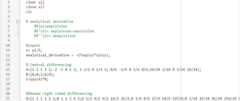
We assign the value of x and range of dx
We define an anonymous function of analytical function and its derivative.
Use the matrices from above discussed section and solved it using inversion method i.e.

AX=B ==> X=A^-1B

And stored the coefficients in cf1, cf2 and cf3.

Assigned the rows and column to the appropriate matrices.
Loop the order of approximation expression in a for loop under the range of dx . Here absolute error is also calculated from the derivative value calculated analytically.

PLOT GRAPH:

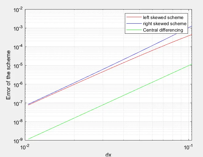
It can be seen from the above plot, the central difference scheme has the lowest error when compared to the right and left-skewed difference methods.
The error values decrease rapidly as the discretization size decreases up to some extent and thereafter, the error starts increasing. This change in the trend of the error is due to the round off error occurring due to computational limits.
Hence while choosing the discretization size, care should be taken to account for round off errors due to computational limits.
Although the central difference method has the lowest error values when compared to skewed method, skewed methods are more useful because we can predict the derivative of a function at a point by knowing the values of the function only on one side of the point (left or right).
This is of greater benefit when we have information about the function on only one side of the point in the numerical stencil. Whereas, the central difference method requires information on both sides of the point in the numerical stencil.

Why skewed scheme is useful? What can a skewed scheme do that a central differencing scheme cannot?

A skewed scheme is useful when we have to predict using the boundary condition as we have only one direction to go. Hence the skewed scheme will be useful and we cannot use the central differencing scheme for such an application because it required information from both directions of the point.

CONCLUSION:

The central differencing scheme has very less error compared to other schemes. Therefore, central differencing is better than other schemes because it uses information from both the sides from the point of consideration to give approximative and accurate values.
As the left and right skewed difference methods uses data only from one side of point of interest it gives less approximative and accurate values about the point.

Week 3.5 - Deriving 4th order approximation of a 2nd order derivative using Taylor Table method

Ship work like this
in your own course.

Talk to a career counsellor

Ship work like thisin your own course.

Talk to a career counsellor

Ship work like this
in your own course.