Week 9 - FVM Literature Review

AIM:

• To explain about Finite Volume Method(FVM)
• To write down the major differences between FDM & FVM.
• Describe the need for interpolation schemes and flux limiters in FVM. By using the 1D linear heat conduction equation as an example.

Finite volume method:

The finite volume method (FVM) is a method for representing and evaluating partial differential equations in the form of algebraic equations. In the finite volume method, volume integrals in a partial differential equation that contain a divergence term are converted to surface integrals, using the divergence theorem. These terms are then evaluated as fluxes at the surfaces of each finite volume. Because the flux entering a given volume is identical to that leaving the adjacent volume, these methods are conservative. Another advantage of the finite volume method is that it is easily formulated to allow for unstructured meshes. The method is used in many computational fluid dynamics packages. "Finite volume" refers to the small volume surrounding each node point on a mesh.

In this method instead of writing the equation in a point, we write it for volume. Then we apply few mathematical techniques to help us solve these equations for any type of grids. Also the finite volume represents preserves the concept of conservation.

The method starts by dividing the flow domain into a number of small control volumes.In the finite volume method, volume integrals in a partial differential equation that contain a divergence term are converted to surface integrals, using the divergence theorem. These terms are then evaluated as fluxes at the surfaces of each finite volume. Because the flux entering a given volume is identical to that leaving the adjacent volume, these methods are conservative.

The advantage of the finite volume method is that it is easily formulated to allow for unstructured meshes, and this method is used in many computational fluid dynamic packages.

Major differences between FDM & FVM:

	Finite Difference Method	Finite Volume Method
GRID GENERATION	The domain is divided into numerous points that are referred to as grid points each of which represents the respective variable of interest.	The domain is divided into numerous control volumes mostly referred to as cells which consist of variables of interest that are located at the centroid of each control volume or cell.
MODE OF DISCRETISATION	The discretization is based on the derivatives since the differential form of governing equations is replaced by a system of algebraic equations at each grid point.	Volume integrals in a PDE that contains a divergence term are then converted into surface integrals by using the divergence theorem. These terms are then evaluated as fluxes at the surfaces of each finite volume.
NUMERICAL SCHEMES	It is applicable in the case of FDM are Forward differencing, Central differencing & Backward differencing.	It is applicable in the case of FVM are Upwind differencing, Hybrid differencing, Power-law which is used for giving a more accurate approximation to the one-dimensional exact solution.

Interpolation schemes in Finite Volume Method:

The interpolation or the approximation schemes are required in the FVM method for the conversion of the integral form of the governing equation to an algebraic equation which can then be solved using various numerical methods. These schemes also play a significant role in the calculation of the values of the flow quantities in the point of concern from the values that are already known from their neighboring faces/cells. Some of the interpolation schemes are listed as follows:

• Upwind Interpolation
• Linear Interpolation
• Quadratic Upwind Interpolation Scheme(QUICK)
• Hybrid, TVD(Total variation dimension) & ENO(Essentially non-oscillatory) interpolation scheme.

Upwind Interpolation Scheme:

• It is mainly used for the convection dominant problems. Velocity for a given point the direction of that velocity that determines the variables values used in interpolation process. In upwind scheme it makes use of nodes that are in the upstream of the given node.
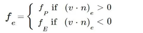
• It is used to calculate the approximate value of the variable(f) at the east face of the control volume, the equation is given by

where ,

f p is the point of the left of face e

f E is the point to the right of face e

(v.n) is Velocity vector

• This scheme is almost like the forward difference approximation or a backward difference approximation based on the flow direction.
• We know that when calculating gradience, we need to have those values bounded, so that they do not jump. Hence this approximation satisfies the boundness condition.

Linear Interpolation Scheme -

Linear interpolation is the method of generating new data points with a range of a discrete set of known data points.

• The linear Interpolation scheme is same as the central difference formula that we considered for the first order derivative. So, this scheme is also known as the central difference scheme.
• Generally, it is used to solve the integrated convection-diffusion equation.It leads to a easy approximation for the evaluation of gradients that are required for evaluation of diffusive fluxes.
• CDS is a second order accurate and may produce oscillatory solutions i.e here if the grid spacing is very large, we can find oscillatory solutions. It is basically a first order, as we refine the grid then accuracy is close to the second order.

Quadratic upwind Interpolation Scheme -

• In CFD it is called as QUICK i.e. Quadratic Upstream Interpolation for Convective Kinematics
• QUICK considers the second order derivative term into consideration and ignores the third order derivative term. Hence it is considered as third order accurate.

Now approximate the value of the variable at the face centre of the control volume by the quadratic interpolation by using the values at three nearest computational nodes i.e. 1 downstream node(D) and two upstream nodes(U, UU) respectively. The equation is given by

This scheme generally used to solve the convective-diffusion equations using the second order central difference for the diffusion term and for the convection term scheme is third order accurate in space and first order accurate in time.

Hybrid Interpolation scheme:

This interpolation method is a blend of both central differencing scheme and Upwind differencing scheme which is based on local peclet number. It can be described by the general partial equation as follows,

Flux Limiters:

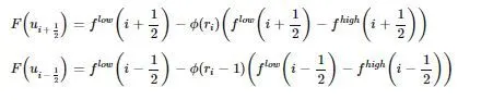
Flux limiters are used in the numerical schemes to solve problems of fluid dynamics, described by highly coupled non-linear Partial Differential Equations. If we tend to use low order numerical schemes for the solving of the governing equations then we might get a highly oscillatory and unstable solution near the discontinuity if present. Whereas if we tend to use higher-order numerical schemes to capture the phenomenon more accurately we tend to exploit the computational power unnecessarily. The main idea behind the use of the flux limiters is to limit the spatial derivative terms near the discontinuities to physical real values so as to maintain physical consistency. There are several types of flux/slope limiter functions. They come in handy when sharp wave-fronts/peaks are present. For smoothly changing waves/functions, the flux limiters do not operate and the spatial derivatives can be represented normally.

It is imperative to note that flux limiters are also referred to as slope limiters because they both have the same mathematical form, and both have the effect of limiting the solution gradient near shocks or discontinuities.

Here,

f low = low precision Flux

f high = High precision Flux