Week 8 - Simulation of a backward facing step in OpenFOAM

AIM:

To simulate an incompressible-laminar-viscous flow through the backward facing step geometry. We should perform a transient simulation. The solver can be chosen based on the described physics of the flow. We need to explain the entire simulation procedure . We should provide explanations to every change we make inside the reference case files obtained from OpenFOAM tutorials. We can choose the inlet velocity such that the flow is laminar.

PROCEDURE:

To simulate an incompressible-laminar-viscous flow through the backward facing step geometry. We consider two cases

Case 1 - Simulate the flow without using any grading factor (i.e., GF = 1)

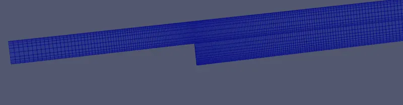
Case 2 - Simulate the flow with grading factor of 0.2. The cells should be finer near the walls (includig the step wall).

Mesh specification

1. Number of cells along the x direction (longer dimension) = 200
2. Number of cells along the longer y direction = 20;

Boundary condition specification

The domain specifications are provided in the following figure.

Grading Factor = Size of the last cell/ Size of the first cell

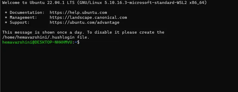
Now in order to start our simulation , we will open the terminal window in ubuntu

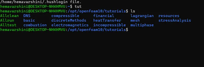
Now, in order to simulate our problem statement in OpenFOAM, we will type 'tut' to open OpenFOAM tutorial directory. Then 'ls' to view all the tutorials present inside this directory.

We have to solve incompressible-laminar-viscous flow simulation for this problem so we will select the 'incompressible' directory by typing 'cd incompressible' and then type 'ls' again to view various folders inside the incompressible directory.

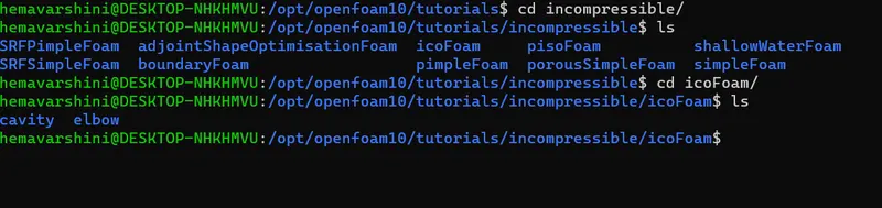
we will select icoFoam folder by typing 'cd icoFoam' and then again we'll type 'ls' to explore that folder in the terminal window.

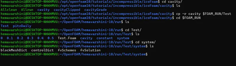
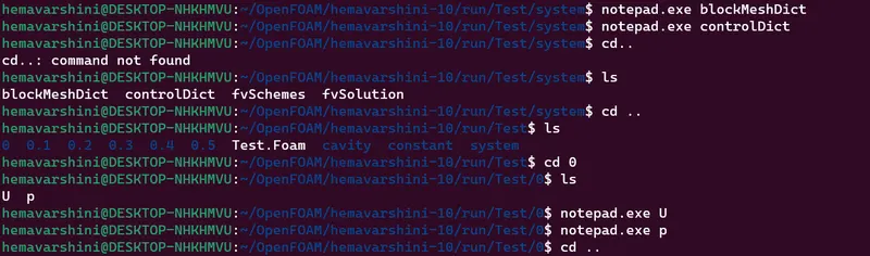
we can see cavity and elbow inside the icoFoam, we will open and see the cavity folder and but we cant make changes to the original tutorial folder as OpenFOAM will not give access to do that , so we will make a copy of that folder using the command 'cp -r cavity' & then we will paste all the directories inside the OpenFOAM's Run folder by typing 'cp -r cavity $FOAM_RUN'/Test'.

We can see all the information copied from the tutorials .we can further see some more directiories inside cavity now which we can change them so that OpenFOAM does not restrict our action.

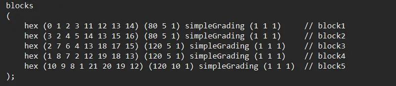
We will open blockMeshDict script file and make changes by using notepad.exe blockMeshDict command

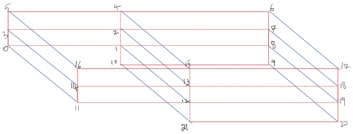
We will refer this image and provide vertices for each and every blockMesh

This is the header file which cannot be changed are executed as per our need

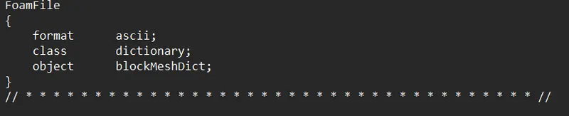
Below image is referred as Dictionary. Which consists of key(format,class,object) and values(ascii,dictionary...) in it

These are the vertices

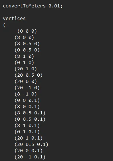
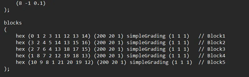
Also we specify the faces as the inlet, outlet ,frontandback and walls

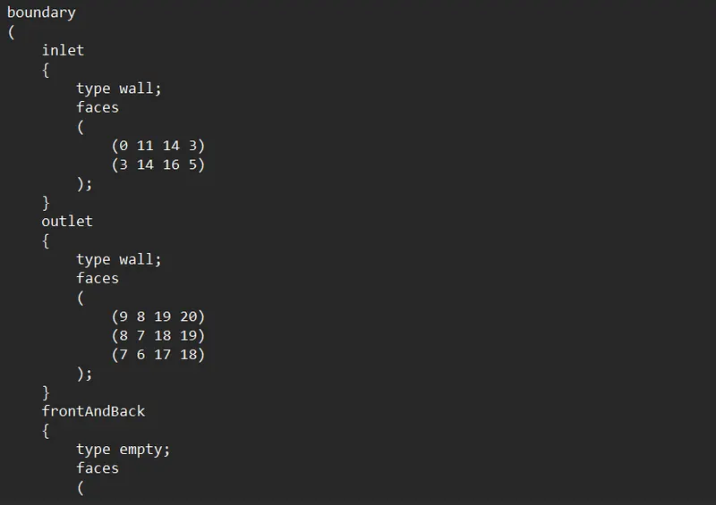
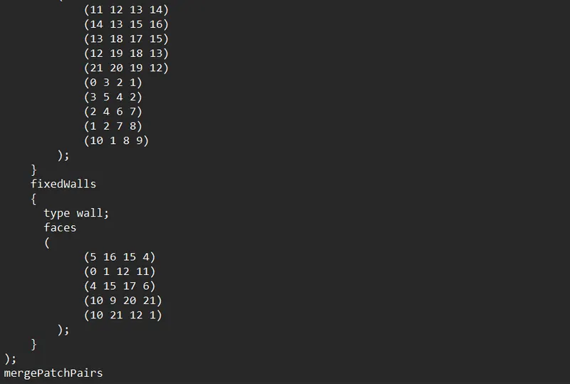
After changing the blockMeshDict script file .We will now change our directory and go to the 'Test' folder in order to go inside a folder named as '0' which consist of two script files, pressure 'P' and velocity 'U'.

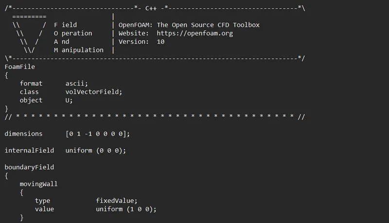
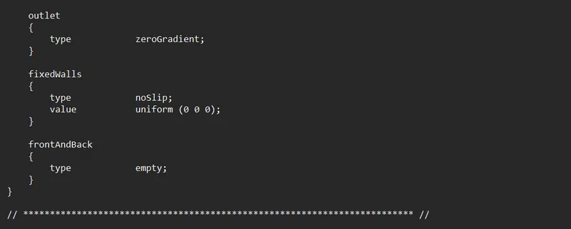
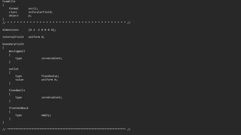
Using Notepad.exe command we can open both velocity and pressure script file and make changes

For Velocity

For Pressure

After making the changes in scriptfile then we are going back to the 'Test' folder and we're going to use the command 'blockMesh' in the terminal to generate our final mesh.

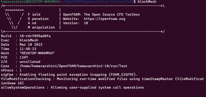
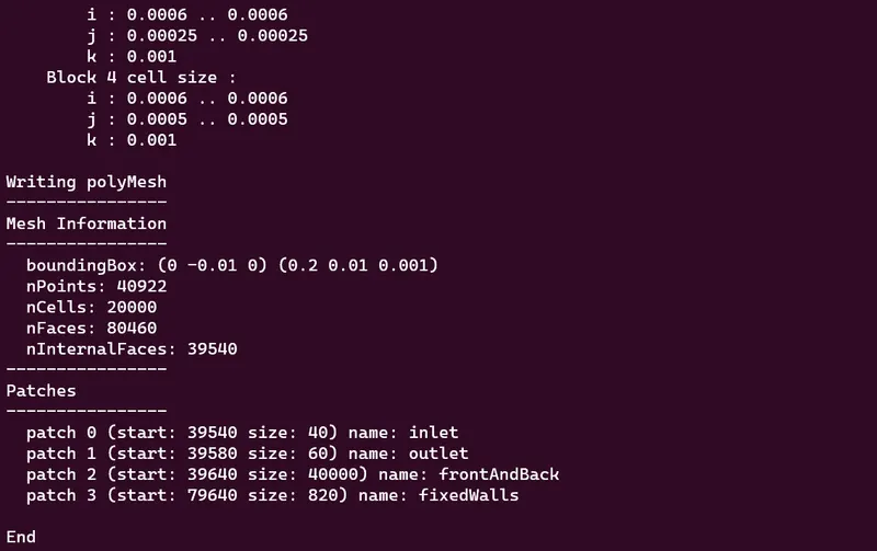
we can see the faces created by OpenFOAM for inlet, outlet, walls and also OpenFOAM has generated faces for defaultFaces in patch 3.

Now we will run a command checkMesh which is used in order to check if the mesh which is being generated above is in appropirate condition or not.

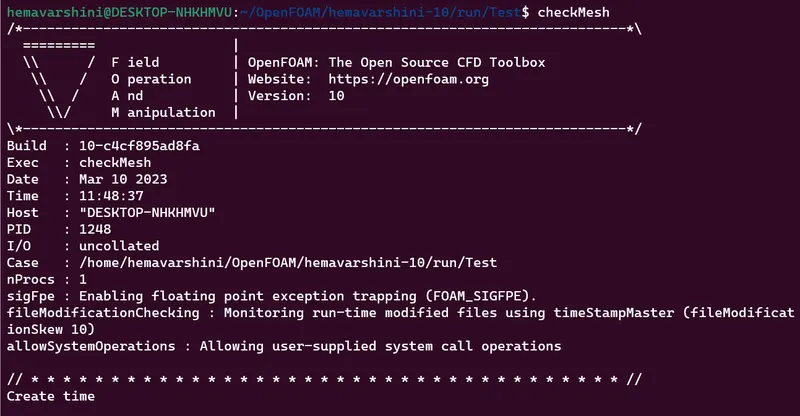
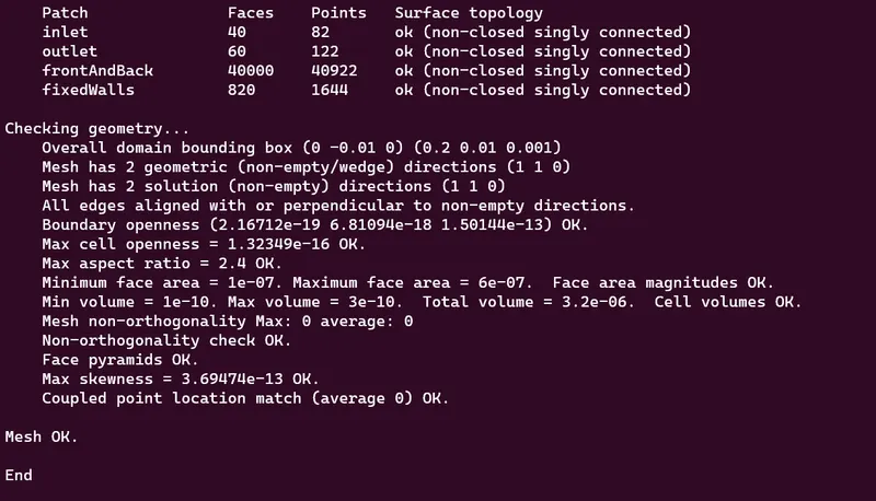
Here,am using explorer.exe . command to open the Test in paraview

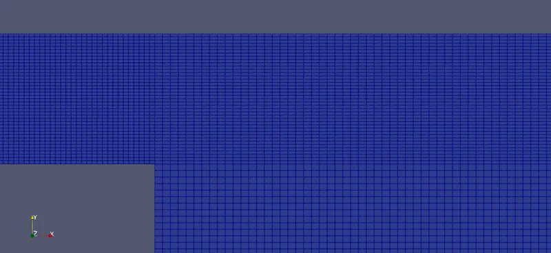
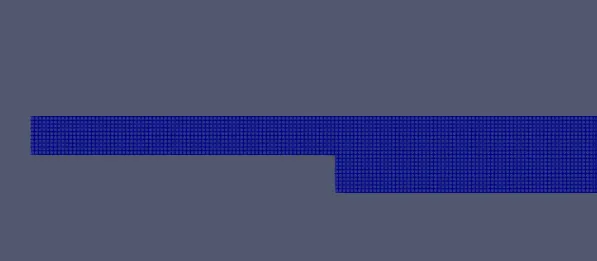
We can notice that it is not uniform all over the surface. So let us just adjust the mesh grid following way.

After deploying mesh, now we are ready to run the simulation. Simulation solver that we have choosen is icoFoam. Hence, just type ‘icoFoam’ and simulation will start.

GRAPHS:

Case 1 - Simulate the flow without using any grading factor (i.e., GF = 1)

Blockmesh:

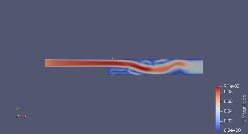
Velocity Distribution:

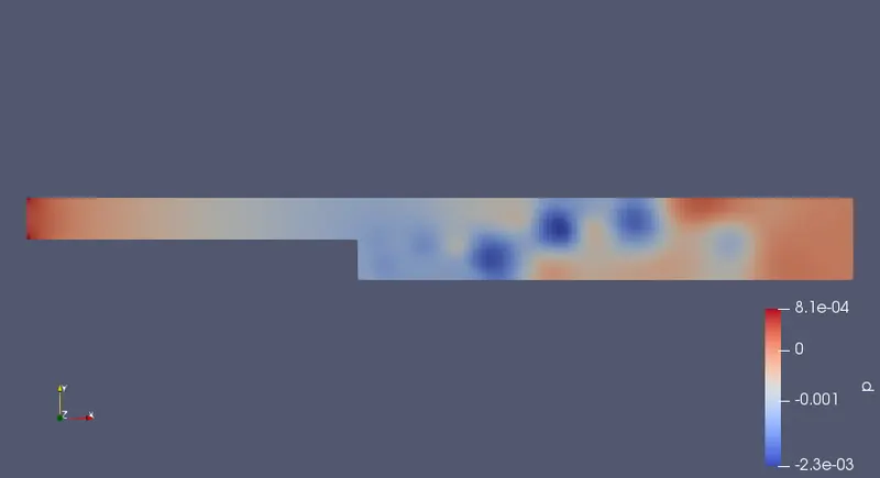
Pressure distribution:

Plot for the velocity profile at 0.085 m

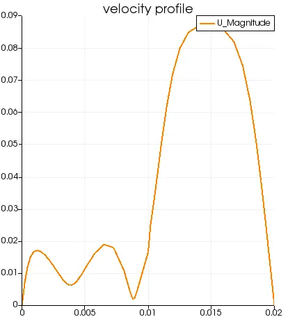
Case 2 - Simulate the flow with grading factor of 0.2. The cells should be finer near the walls (includig the step wall).

Blockmesh:

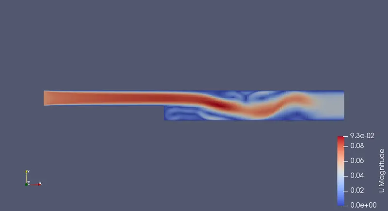
Velocity Distribution:

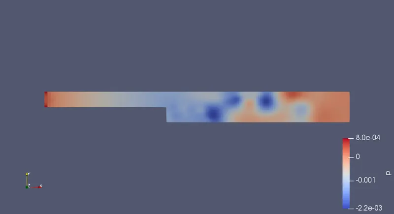
Pressure distribution:

Plot for the velocity profile at 0.085 m

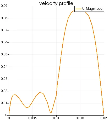
By comparing the results obtained from both the cases we conclude that the results obtained are approximately same but the execution time for case 2 is slightly higher than case 1 .

Case 1 seems to be more accurate & smoother than the case 2. Hence, we can observe that when the mesh is not uniform, it can disrupt our output results to some extent.

Mesh-grid needs to be finer in order to capture the flow properties with better accuracy as shown in the case 1 as the mesh is uniform at all section.

Why Grading/Growth factor is essential for meshing.

• In computational fluid dynamics the grading is useful for computational efficiency. In CFD fluid always shows the largest changes in near the walls or obstacles so in order to capture that changes we always use fine mesh near the wall.
• Grading factor actually helps us to adjust the sizes of the respective cells from the initial section of the block to the final section of that block.
• To get the effective and reliable results. we have to know where to use fine grading factor . For obtaining the more effective results, if we use large number of fine elements in mesh,It could increases the computational time for converging the solution but it is helpful to capture the flow at boundary walls and obstacles.

CONCLUSION:

• Simulation is done on an incompressible-laminar-viscous flow through the backward facing step geometry and also performed a transient simulation.By choosing the solver based on the described physics of the flow.
• Explained the entire simulation procedure .By providing explanations to every change you make inside the reference case files obtained from OpenFOAM tutorials. choosed the inlet velocity shuch that the flow is laminar.
• Performed 2 case studies with grading and without grading and also compared the results.
• Plotted graph for the velocity profile at 0.085 m