Week 5.1 - Mid term project - Solving the steady and unsteady 2D heat conduction problem

Obejctive:- To write code to solve 2D heat conduction equastion by iterative solver techniques.

Theory:- Generalized Heat conduction equation for 2D space

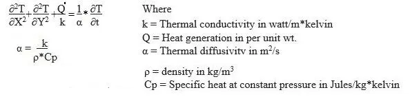
Here, thermal diffusitivity is ratio of Conductivity and Heat capacity which mean α signifies the ability of a substance to conduct heat relative to its ability to store thermal energy.

Conducitivity mean how Tempratre is distributing inside a Solid block and diffusitivity mean how much heat spread by a molecule to nearby molecules after abosorbing heat.

There are two modes of solving this 2D heat conduction equation

1). Transient Mode

If there is no heat generation then 2D Generalized Heat conduction equation is

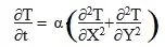
This is a time dependent second order PDE of 2D space so, it is called as Transient analysis.

Here temperature profile depends on both time and space.

Now we solve this PDE numerically by using first order forward differencing scheme for first order time derivative and Central differencing scheme for 2^nd order space

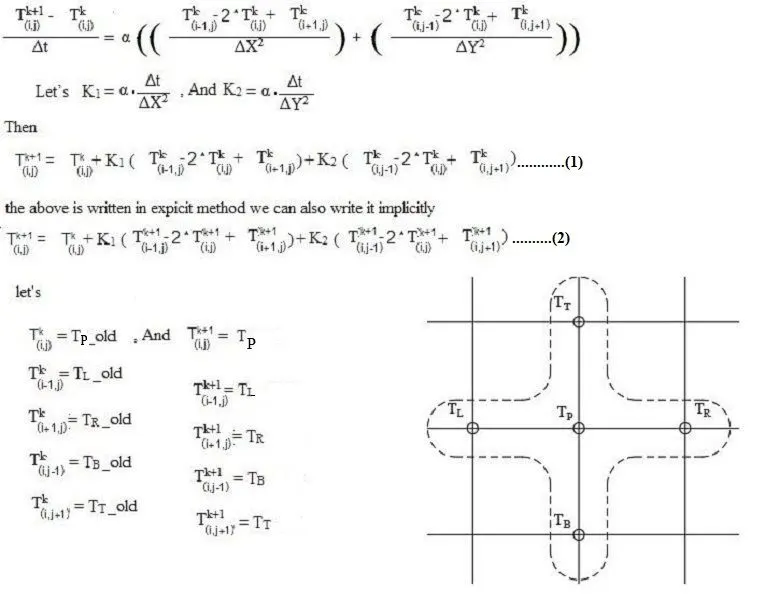
Explicit method:-

Now after substituting above notation in our above expression

then equastion (1) will be

Tp=Tp_old+K1*(TL_old-2*Tp_old+TR_old)+K2*(TB_old-2*Tp_old+TT_old)

Tp=(1-2*K1-2*K2)*Tp_old+K1*(TL_old+TR_old)+K2*(TB_old+TT_old)

Now,

here T_old represent Temperature profile in privious time step and T represent Temperature profile this time step, or in our equastion (1) power k represent privious generation for time step.so k+1 is current generation or current time step where as k is privious time step.

As we observe in above expression and equastion (1), the current generation temperature value in the LHS and privious temperature values in RHS of the equastion.so it called explict solution.we can futher write our equastion in below the terms

term_1=(1-2*K1-2*K2)*Tp_old=(1-2*K1-2*K2)*T_old(i,j)

term_2=K1*(TL_old+TR_old)=K1*(T_old(i-1,j)+T_old(i+1,j))

term_3=K2*(TB_old+TR_old)=K1*(T_old(i,j-1)+T_old(i,j+1))

then

T(i,j)=term_1+term_2+term_3

Matlab code for Explicit Transient Mode

Step 1:- First give inputs grid size and time steps and also give Thermal diffusivityof system such that it satisfied CFL condition for 2D space i.e.

CFL_x+CFL_y=CFL<0.5

Define 2D grid space and time space

Step 2:- Assining B.C. and creating initial temprature profile

Step 3:- Define constant values as per theory

Step 4:- Time Loop

before the time loop define initial time by tic

Define initial error and tol for Iterative Loop in side time loop

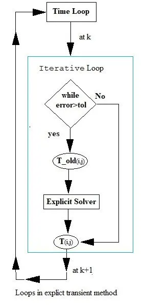
Step 5:- Iterative Loop or while loop

inside this loop de define space loop where we calculate new Temperature matrix for and then calculate error in while loop, if error>tol then this loop again runs and space loop inside it also runs which gives again a new Temperature matrix and this will be continue untill error<tol.

Note;-error=max of abs (T-T_old)

1. here T_old is Temperature matrix of last iteration and it has to update befor end of the while loop.
2. but when in time loop T_old is Temperature matrix for old time step and this Iterative Loop is inside the Time loop and runs for each value of time steps nor each value of k.so when it run for 2st iteration in any time step k+1 it take T_old vlaue of last iteration of time step k.
3. And then for 2nd iteration it takes T_old vlaue of 1st iteration of time step k+1.
4. so here we update T_old value only inside the while loop.because in explicit method expression the RHS values are only from priviuous time step.so we update for both Next iteration and time step only inside bthe while loop.

Step 6:- Space Loop

here we define expression of T(i,J) and all the terms from above theory and here we use T_old matrix elements only as input for generation new T matrix for each point in 2D grid space.

% Code to solve explicitly a Transient 2D Heat Conduction equastion without heat genration
clear all
close all
clc
% Imputs
% Number of nodes in 2D space
nx=10;
ny=nx;
nt=1400; % Number of time steps
alpha=1.4; % Thermal diffusity is set such that CFL<0.5

% Creating 2D space
x=linspace(0,1,nx);
y=linspace(0,1,ny);

% Defning mesh or grid size in 2D space
dx=x(2)-x(1);
dy=dx;
dt=1e-3; % AS our alpha and dx given already so for stable solution

% Assining B.C. and creating initial temprature profile
TL=400;
TT=600;
TR=800;
TB=900;
T=300*ones(nx,ny);

T(2:ny-1,1)=TL;
T(2:ny-1,nx)=TR;
T(1,2:nx-1)=TT;
T(ny,2:nx-1)=TB;
% Calculating average temperature for cornear grids
T(1,1)=(TT+TL)/2;
T(nx,ny)=(TR+TB)/2;
T(1,ny)=(TR+TT)/2;
T(nx,1)=(TL+TB)/2;

% Assining orginal values of T
T_initial=T;
T_old=T;

% Definig  constant
K1=alpha*dt/dx^2;
K2=alpha*dt/dy^2;

% Time Loop
iter=1;
tic
for k=1:nt
    % Iterative Loop
    % Define convergion criteria for Iterative Loop
    tol=1e-4;
    error=9e9; % Initially Higher then tol.
    % Call Solution is converged
    while(error>tol)
        for i=2:nx-1
            for j=2:ny-1
                term_1=(1-2*K1-2*K2)*T_old(i,j);
                term_2=K1*(T_old(i-1,j)+T_old(i+1,j));
                term_3=K1*(T_old(i,j-1)+T_old(i,j+1));
                T(i,j)=term_1+term_2+term_3;
            end
        end
        % Calculating error
        error=max(max(abs(T_old-T)));
        % Updating iter
        iter=iter+1;
        % Updating old value for next time step
        T_old=T;
    end
end
% Calculating Simulation Time
time=toc;
% Temperature ploting
figure(2)
T_trans=flip(T);
contourf(x,y,T_trans)
clabel(contourf(x,y,T_trans))
colorbar
colormap(jet)
xlabel('X-Axis')
ylabel('Y-Axis')
title_Text_1=sprintf('Number of Iteration =%d',iter);
title_Text_2=sprintf('Number time step= %d',k);
title_Text_3=sprintf('Total Simulation Time in second = %d',time);
title({title_Text_1,title_Text_2,title_Text_3})
pause(0.03) 

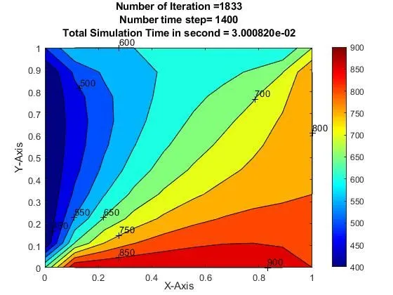
Result

Implicit method:-

Now after substituting above notation in our above expression

then equastion (2) will be

Tp=Tp_old+K1*(TL-2*Tp+TR)+K2*(TB-2*Tp+TT)

Tp+K1*2*Tp+2*Tp=Tp_old+K1*(TL+TR)+K2*(TB+TT)

Tp=(Tp_old+K1*(TL+TR)+K2*(TB+TT))/(1+2*K1+2*K2)

here T_old represent Temperature value of privious time step and Tp,TL,TR,TT and TB are Temperature value of current time step. and when we required values of Tp,TL,TR,TT and TB for last Iteration so i use T_old, TL_old, TR_old, TT_old and TB_old instade of Tp, TL,TR,TT and TB.

now i use T_prv_dt for emperature value of privious time step in stade of T_old because be use T_old for Tp of last iteration.

then our expression is

Tp=(T_prv_dt+K1*(TL+TR)+K2*(TB+TT))/(1+2*K1+2*K2)

Now we ca write

term_1=(1+2*K1+2*K2)^(-1)

term_2=K1*term_1

term_3=K2*term_1

and

H=(TL+TR)=(T(i-1,j)+T(i+1,j))

V=(TT+TB)=(T(i,j-1)+T(i,j+1))

T(i,j)=T_prv_dt(i,j)*term_1+H*term_2+V*term_3

Now this Implicit equation can solve future in 3 ways

1). Jacobi method

2). Gause seidel method

and 3). Successive over-relaxation Method

1). Jacobi method :-In numerical linear algebra, the Jacobi method is an iterative algorithm for determining the solutions of a stricly Diagonally dominant system of linear equations . Each diagonal element is solved for, and an approximate value is plugged in. The process is then iterated until it converges.Jacobi Method is also known as the simultaneous displacement method.

here we cand write system of linear equations in terms of matrix

[A]*[x]=[b]

then solution of this for next iteration

X⁽ⁿ⁺¹⁾ =D^-1(b-R(Xⁿ))

Here D is diagonal foam of matrix A

R is foam of matrix A excluding diagonal elements.Here R take old value of x.

then in or in our implicit expression of 2D heat conduction

H=(T_old(i-1,j)+T_old(i+1,j))

V=(T_old(i,j-1)+T_old(i,j+1))

2).Gause seidel method :-This is s similar to the Jacobi method. Though it can be applied to any matrix with non-zero elements on the diagonals, convergence is only guaranteed if the matrix is either strictly diagonally dominant.but here change is that in jacobi takes value of x from last iteration for all element of R but in Gause seidel we take new value of x for those element R solved in current iteration.

X_i⁽ⁿ⁺¹⁾ =D^-1(b-R(X_(i-1) ⁿ⁺¹) - R(X_(i)ⁿ))

then in or in our implicit expression of 2D heat conduction

H=(T(i-1,j)+T_old(i+1,j))

V=(T(i,j-1)+T_old(i,j+1))

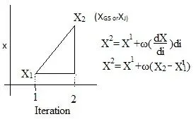
3). Successive over-relaxation Method:- This is a variant of the Gauss–Seidel method for solving a linear system of equations Here we have a shape factor (ω).which is heplful to get resulting in faster convergence.

then

X²= ω * X²_{Gause seidel} + (1-ω)*X¹

^{here ω is scaling factor which is slope of X1X2}

^{if ω>1 more aggressively change so it is called as over relaxation}

^{if ω>1 less aggressively change so it is called as under relaxation}

T_(i,j)=SF*T_GS_(i,j)+(1-SF)*T_old_(i,j)

Matlab code for Implicit Transient Mode

Initial three steps are same as Explict Transient.

Step 4:-Now we have to select of solver method i.e. jacobi,gause seidel and SOR

Here we use a input function through which we can select our method in command window.This command use to input value of varible iterative_solver=1,2or3 which represent jacobi,gause seidel and SOR methods respectivly.

now we apply if loop for each method where we say if iterative_solver==1 it run code only for jacobien and similary for others.

Step 5:- Time Loop

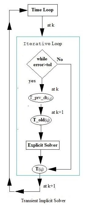
Now in each if loop there is a time loop which is similary to expcit method where is a iterative loop in side the time loop.but in Implicit method the diffrence is that after completing the while loop there is update of T_prv_dt matrix for each time Loop.

**Note:- error is define inside the time loop befor the while because if we define it out side the time loop after compliting while loop error

This proble also occure in Explit solver but in implict solver it give more seviour effect on solution.**

Step 5:- Iterative Loop or while loop this similar to explict method it contains a spsce loop inside it.and here we update T_old for next iteration only not for next time step for next we have T_prv_dt update in time loop.

Step 6:- Space Loop

here we define expression of T(i,J) and all the terms from above theory and here we use T_old matrix (which update in each while loop) and T_prv_dt matrix (which update in each time loop) +

Step 7:- Plotting result

% Code to solve Implicitly a Transient 2D Heat Conduction equastion without heat genration
clear all
close all
clc
% Imputs
% Number of nodes in 2D space
nx=10;
ny=nx;
t=1000;
dt=1e-3; % AS our alpha and dx given already so for stable solution
nt=1400; % Number of time steps
alpha=1.4; % Thermal diffusity is set such that CFL<0.5
% Scale factor for Successive over-relaxation is grater then unity
SF=1.2 ;

% Creating 2D space
x=linspace(0,1,nx);
y=linspace(0,1,ny);

% Defning mesh or grid size in 2D space
dx=x(2)-x(1);
dy=dx;
% Assining B.C. and creating initial temprature profile
TL=400;
TT=600;
TR=800;
TB=900;
T=300*ones(nx,ny);

T(2:ny-1,1)=TL;
T(2:ny-1,nx)=TR;
T(1,2:nx-1)=TT;
T(ny,2:nx-1)=TB;
% Calculating average temperature for cornear grids
T(1,1)=(TT+TL)/2;
T(nx,ny)=(TR+TB)/2;
T(1,ny)=(TR+TT)/2;
T(nx,1)=(TL+TB)/2;

% Assining orginal values of T
T_initial=T;
T_old=T; % Temperature profile for privious itteration 
T_prv_dt=T; % Temperature profile for privious time step

% Definig constant terms
K1=alpha*dt/dx^2;
K2=alpha*dt/dy^2;

% Input display
disp('Select method for solving 2D steady state heat conduction equastion')
disp('iterative_solver = 1 for Jacobi Method')
disp('iterative_solver = 2 for Gause-seidel Method')
disp('iterative_solver = 3 for Successive over relaxation Method')
iterative_solver=input('iterative_solver:');

% Jacobi Method

if iterative_solver==1
    jacobi_iter=1;
    tic
    % Time Loop
    for k=1:nt
        % Iterative Loop
        % Define convergion criteria
        tol=1e-4; % Call Solution is converge
        error=9e9; % Initially Higher then tol.
        while(error>tol)
             for i=2:nx-1
                for j=2:ny-1
                    term_1=(1+(2*K1)+(2*K2))^(-1);
                    term_2=K1*term_1;
                    term_3=K2*term_1;
                    H=(T_old(i-1,j)+T_old(i+1,j));
                    V=(T_old(i,j-1)+T_old(i,j+1));
                    T(i,j)=(T_prv_dt(i,j)*term_1)+(H*term_2)+(V*term_3);
                end
             end
            % Calculating error
            error = max(max(abs(T_old-T)));
            % Updating old value of T for next Iteration time step
            T_old=T;
            % Calculating iter
            jacobi_iter=jacobi_iter+1;
        end
        % Updating old value of T for next step
        T_prv_dt = T;
    end
    time=toc
    % Temperature ploting
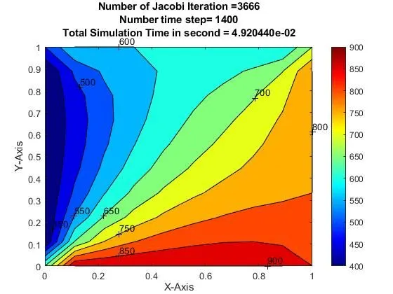
    figure(1)
    T_j=flip(T);
    contourf(x,y,T_j)
    clabel(contourf(x,y,T_j))
    colorbar
    colormap(jet)
    xlabel('X-Axis')
    ylabel('Y-Axis')
    title_J1=sprintf('Number of Jacobi Iteration =%d',jacobi_iter);
    title_J2=sprintf('Number time step= %d',k);
    title_J3=sprintf('Total Simulation Time in second = %d',time);
    title({title_J1,title_J2,title_J3})
    pause(0.03)
end

% Gauss-seidel Method

if iterative_solver==2
    Gauss_seidel_iter=1;
    tic
    % Time Loop
    for k=1:nt
        % Iterative Loop
        % Define convergion criteria
        tol=1e-4; % Call Solution is converge
        error=9e9; % Initially Higher then tol.
        while(error>tol)
             for i=2:nx-1
                for j=2:ny-1
                    term_1=(1+(2*K1)+(2*K2))^(-1);
                    term_2=K1*term_1;
                    term_3=K2*term_1;
                    H=(T(i-1,j)+T_old(i+1,j));
                    V=(T(i,j-1)+T_old(i,j+1));
                    T(i,j)=(T_prv_dt(i,j)*term_1)+(H*term_2)+(V*term_3);
                end
             end
            % Calculating error
            error = max(max(abs(T_old-T)));
            % Updating old value of T for next Iteration time step
            T_old=T;
            % Calculating iter
            Gauss_seidel_iter=Gauss_seidel_iter+1;
        end
        % Updating old value of T for next step
        T_prv_dt = T;
    end
    time=toc
    % Temperature ploting
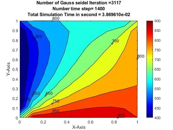
    figure(2)
    T_G=flip(T);
    contourf(x,y,T_G)
    clabel(contourf(x,y,T_G))
    colorbar
    colormap(jet)
    xlabel('X-Axis')
    ylabel('Y-Axis')
    title_G1=sprintf('Number of Gauss seidel Iteration =%d',Gauss_seidel_iter);
    title_G2=sprintf('Number time step= %d',k);
    title_G3=sprintf('Total Simulation Time in second = %d',time);
    title({title_G1,title_G2,title_G3})
    pause(0.03)
end

% Successive over-relaxation Method

if iterative_solver==3
    SOR_iter=1;
    tic
    % Time Loop
    for k=1:nt
        % Iterative Loop
        % Define convergion criteria
        tol=1e-4; % Call Solution is converge
        error=9e9; % Initially Higher then tol.
        while(error>tol)
             for i=2:nx-1
                for j=2:ny-1
                    term_1=(1+(2*K1)+(2*K2))^(-1);
                    term_2=K1*term_1;
                    term_3=K2*term_1;
                    H=(T(i-1,j)+T_old(i+1,j));
                    V=(T(i,j-1)+T_old(i,j+1));
                    T_GS(i,j)=(T_prv_dt(i,j)*term_1)+(H*term_2)+(V*term_3);
                    T(i,j)=(SF*T_GS(i,j))+((1-SF)*T_old(i,j));
                end
             end
            % Calculating error
            error = max(max(abs(T_old-T)));
            % Updating old value of T for next Iteration time step
            T_old=T;
            % Calculating iter
            SOR_iter=SOR_iter+1;
        end
        % Updating old value of T for next step
        T_prv_dt = T;
    end
    time=toc
    % Temperature ploting
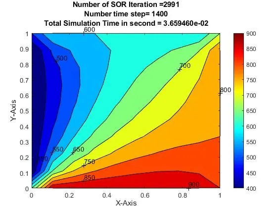
    figure(3)
    T_S=flip(T);
    contourf(x,y,T_S)
    clabel(contourf(x,y,T_S))
    colorbar
    colormap(jet)
    xlabel('X-Axis')
    ylabel('Y-Axis')
    title_S1=sprintf('Number of SOR Iteration =%d',SOR_iter);
    title_S2=sprintf('Number time step= %d',k);
    title_S3=sprintf('Total Simulation Time in second = %d',time);
    title({title_S1,title_S2,title_S3})
    pause(0.03)
end

Result:-

2). Steay state Mode:-In our 2d heat conduction equation if heat generation and time derivative of Temperature are Zero, then

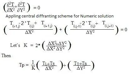
K_x=1/K*dX²

K_y=1/K*dY²

term_1=Kx(T_(i-1,j)+ T_(i+1,j))

term_2=Ky(T_(i,j-1)+ T_(i,j+1))

T_(i,j)=term_1+term_2

Now this Implicit equation can solve future in 3 ways

1). Jacobi method

term_1=Kx(T_old_(i-1,j)+ T_old_(i+1,j))

term_2=Ky(T_old_(i,j-1)+ T_old_(i,j+1))

T_J_(i,j)=term_1+term_2

2). Gause seidel method

term_1=Kx(T_(i-1,j)+ T_old_(i+1,j))

term_2=Ky(T_(i,j-1)+ T_old_(i,j+1))

T_GS_(i,j)=term_1+term_2

3). Successive over-relaxation Method

T_SOR_(i,j)=SF*T_GS_(i,j)+(1-SF)*T_old_(i,j)

Matlab code for Implicit Transient Mode

Step 1:- First give inputs grid size and define 2D grid space with linspace command

Step 2:- Assining B.C. and creating initial temprature profile

Step 3:- Define constant values as per theory

Step 4:-Now we have to select of solver method i.e. jacobi,gause seidel and SOR

so we use input command where we input the iterative solver value in command window as per this value our define if loop is running for jacobi,gause seidel and SOR.

Step 5:-Now each if loop contain a Iterative Loop with condition (error > tol)

in side the while there are Space Loop with the expression of T(i,j)

in each if Loop the expression of this T(i,j) is as per the method and writen for above theory.

if error > tol then this while loop run again again until error <tol

Step 6:- Plotting result

% Code to solve a steady state 2D Heat Conduction equastion without heat genration

clear all
close all
clc
% Imputs
% Number of nodes in 2D space
nx=10;
ny=nx;
% Creating 2D space
x=linspace(0,1,nx);
y=linspace(0,1,ny);

% Defning mesh or grid size in 2D space
dx=x(2)-x(1);
dy=dx;

% Assining B.C. and creating initial temprature profile
TL=400;
TT=600;
TR=800;
TB=900;
T=300*ones(nx,ny);

T(2:ny-1,1)=TL;
T(2:ny-1,nx)=TR;
T(1,2:nx-1)=TT;
T(ny,2:nx-1)=TB;
% Calculating average temperature for cornear grids
T(1,1)=(TT+TL)/2;
T(nx,ny)=(TR+TB)/2;
T(1,ny)=(TR+TT)/2;
T(nx,1)=(TL+TB)/2;

% Assining orginal values of T
T_initial=T;
T_old=T;

% Define convergion criteria
tol=1e-4; % Call Solution is converged
error=9e9; % Initially Higher then tol.

% Scale factor for Successive over-relaxation is grater then unity
SF=1.2 ;

% Definig constant terms
K=2*(dx^2+dy^2)/(dx^2*dy^2);
% term 1 is :- kx=1/(K*dx^2)
% term 2 is :- ky=1/(K*dy^2)
kx=1/(K*(dx^2));
ky=1/(K*(dy^2));

% Input display
disp('Select method for solving 2D steady state heat conduction equastion')
disp('Method 1 - Jacobi')
disp('Method 2 - Gause-seidel')
disp('Method 3 - Successive over relaxation')
iterative_solver=input('Method:');


% Jacobi Method

if iterative_solver==1
    jacobi_iter=1;
    tic
    while(error>tol)
         for i=2:nx-1
             for j=2:ny-1
                 term_1=kx*(T_old(i-1,j)+T_old(i+1,j));
                 term_2=ky*(T_old(i,j-1)+T_old(i,j+1));
                 T(i,j)=term_1+term_2;
             end
         end
         % Calculating error
         error=max(max(abs(T_old-T)));
         % Updating old value
         T_old=T;
         jacobi_iter=jacobi_iter+1;
    end
    time=toc;
   % Temperature ploting
   figure (1)
   T_jacobi=flip(T);
   contourf(x,y,T_jacobi)
   clabel(contourf(x,y,T_jacobi))
   colorbar
   colormap(jet)
   xlabel('X-Axis')
   ylabel('Y-Axis')
   title_1=sprintf('Number of Jacobi Iteration in steady state =%d',jacobi_iter);
   title_2=sprintf('Simulation Time in second = %d',time);
   title({title_1,title_2})
   pause(0.03)
end

% Gauss-seidel Method

if iterative_solver==2
    GS_iter=1;
    tic
    while(error>tol)
         for i=2:nx-1
             for j=2:ny-1
                 term_1=kx*(T(i-1,j)+T_old(i+1,j));
                 term_2=ky*(T(i,j-1)+T_old(i,j+1));
                 T(i,j)=term_1+term_2;
             end
         end
         % Calculating error
         error=max(max(abs(T_old-T)));
         % Updating old value
         T_old=T;
         GS_iter=GS_iter+1;
    end
    time=toc;
    % Temperature ploting
    figure(2)
    T_GS=flip(T);
    contourf(x,y,T_GS)
    clabel(contourf(x,y,T_GS))
    colorbar
    colormap(jet)
    xlabel('X-Axis')
    ylabel('Y-Axis')
    title_1=sprintf('Number of Gauss-seidel Iteration in steady state =%d',GS_iter);
    title_2=sprintf('Simulation Time in second = %d',time);
    title({title_1,title_2})
    pause(0.03)
end

% Successive over-relaxation Method
  
if iterative_solver==3
   
   SOR_iter=1;
   I_SOR=[];
   tic
   while(error>tol)
        for i=2:nx-1
             for j=2:ny-1
                 term_1=kx*(T(i-1,j)+T_old(i+1,j));
                 term_2=ky*(T(i,j-1)+T_old(i,j+1));
                 T_GS(i,j)=term_1+term_2;
                 T(i,j)=SF*(T_GS(i,j))+((1-SF)*(T_old(i,j)));
             end
        end
        % Calculating error
        error=max(max(abs(T_old-T)));
        
        % Updating old value
        T_old=T;
        SOR_iter=SOR_iter+1;
    end
    time=toc;
    % Temperature ploting
    figure(3)
    T_SOR=flip(T);
    contourf(x,y,T_SOR)
    clabel(contourf(x,y,T_SOR))
    colorbar
    colormap(jet)
    xlabel('X-Axis')
    ylabel('Y-Axis')
    title_1=sprintf('Number of Successive over-relaxation Iteration in steady state =%d',SOR_iter);
    title_2=sprintf('Simulation Time in second = %d',time);
    title({title_1,title_2})
    pause(0.03)
end

Results plot:-

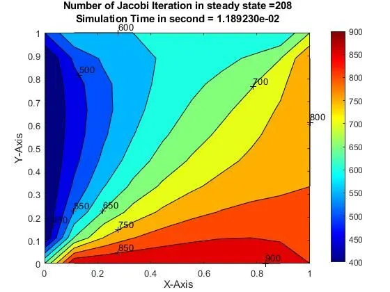
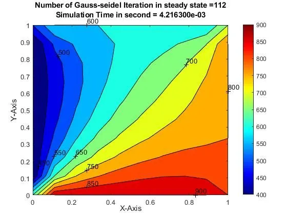
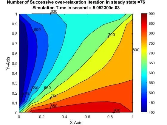
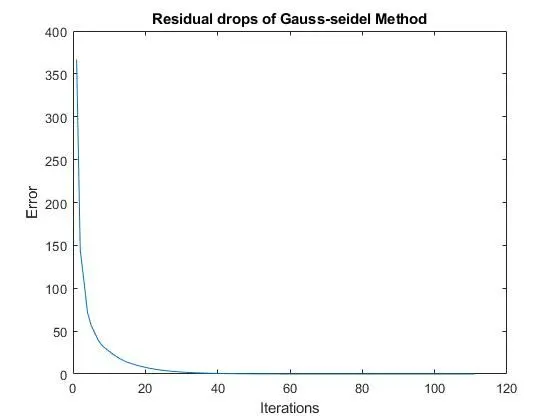
Result Summery

1) From the above plot we observe that resulting Teperature profile is same in all plot but diffrence in Iteration and simulation time.

If we look at the Steady state result for the each method number of iterationis less as compaire to Transient.

S.No.	Method	No. of Iteration	Total simulation time (in sec)
1	Steady state Implicit Jacobi method	208	1.89e-02
2	Steady state Implicit Gause Seidel method	112	4.216e-03
3	Steady state Implicit Successive over-relaxation method	76	5.052e-03
4	Transient Implicit Jacobi method	3666	4.920e-02
5	Transient Implicit Gause Seidel method	3117	3.869e-02
6	Transient Implicit Successive over-relaxation method	2991	3.659e-02
7	Transient Explicit method	1833	3.000e-02

Now if we observe in tabel Transient analysis takes 17 to 40 more iteraion as compaired to their respective Steady state analysis. This is because in teansient mode the itrative loop runs for each value of time step so that number of iteration of cuurent time step are add to the number of iteration of next time step and this will continu until the last time step and we get higher number of iteration at the end.

And if we look at simulation time it is also much more in Transient analysis because each iteration take time to execution and in transient mode no. iterations are more so it takes more time as compare to Steady state.

If we look at explict method it take quit less iteration and simulation time as compared to Implicit method.

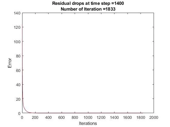
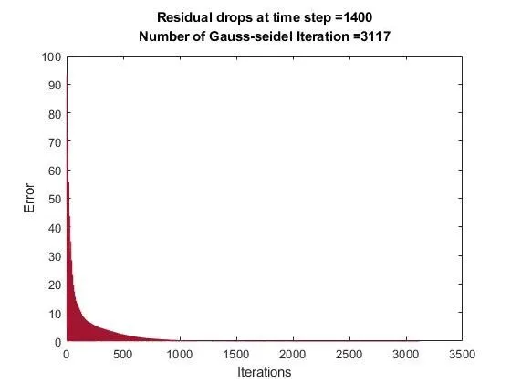
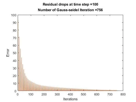
2) If we plot convergence plot for transient and steady state analysis, we can in S.S. Residual drops is a single graph because in ss itrative loop runs till the convergence condition but in transient method if it runs in current time step and get convergence condition then it runs for next time step by taking initial value of error.

If compare Explicit and Implicit method we observed that in explicit transient Residual drops like steeply decline hyperbolic curve, where error is high initialy and decrising very fast upto 200 no. of iteration but after that it looks like a straight line upto last iteration and similar graph we can see in implicit steady state methods only diffrence is in ss it is a single graph and in explict it is a multiple graph.but if we look at implicit Transient graph we can see it is a zic zack graph decline hyperbolically this is because in Implicit transient analysis Itrative solver use Temperature value from last iteration and from last time step also so that in a single time step error value is high for initial iteration and drops faster in that time step and for next time step it again go to higher value (because initial error is high) and drop again. this phenomenal is continue untill the last time step but at the end each time error is decline hyperbolically that can be see in plot.

3) Now, if compare our three method for solving implicit equastion we observed that jacobi method take more iteration as compare to gause seidel and gause seidel take more iteration as compaire to Successive over-relaxation method. This is because in jacobi iteration we take old value of T for all skewed points near to our point of interest but in gause seidel we take old value of T for only those point whose vlaue not calculated yet for cuurnt itration.So we can say Gause seidel take updated value for some point and because of this we get convergance condition in less iteration as compare to jacobi.

5) Successive over-relaxation method have less no of iteration as compare to others.It is because in this method we consider a our slope with multiples with a constant called shape factor. If we increse value of scaling factor then we get more less no of iteration for getting convergance condition because as change in each iteration is more aggressively so we get convergance condition in less iteration.

4) Here for stability of Numeric solution we have CFL condition which expresses that the distance that any information travels during the timestep length within the mesh must be lower than the distance between mesh elements.

CFL=CFL1+CFL2

here for stability of Numeric solution CFL<0.5

CFL1 is for horizontal direction and equal to α*dt/dx²

and , CFL2 is for vertical direction and equal to α*dt/dy²

Now here we can say that CFL not only depend on time step and grid ,it also depend on Thermal diffusivity.

and physical significance of α is how fast heat is spread inside a material.if α is high materical take less time to get into thermal equllibrim condition.if α is low materical take more time to get into thermal equllibrim condition.

So here we have to choose α and dt in such a way our simulation is stable or time for conduction is also not so much.

α=1.4 and dt=1e-3 and CFL=0.23 and time for conduction is 0.14 s

Conclusion:-

1) Number of iteration in Successive over-relaxation is minimum as compare to others because here change is more aggressively in each iteration. and Successive over- relaxation give result faster as compare to other method and jacobi give result slowly as compare to others.

2) Number of iteration and simulation time are inversly perposnal to scaling factor.

3) Steady sate analysis is much faster then Transient because it don't consider effect with respect to time.

4) Implicit method take more no of iteration and time as compare to explicit method.

5) As SS implicit is much faster then transient implicit, so first we do SS analysis and use its result for initial condition for transient analysis to get result much faster and accurate.