Week 7 - Simulation of a 1D Super-sonic nozzle flow simulation using Macormack Method
Aim :- To simulate the isentropic flow through a quasi 1D subsonic-supersonic nozzle.
Objectives:-
- To derive both the conservation and non-conservation forms of the governing equations quasi 1D subsonic-supersonic nozzle flow and sovle them using the MacCormack's technique.
- To determine the steady-state distribution for the flow-field variables for initial and final time step for both forms.
- To explain difference between the conservation and non-conservation forms of governing equations by comparing their numeric solutions and plots.
Theory:-
In this study we consider isentropic flow through a convergent-divergent nozzle as shown in figure(1).Here at nozzle inlet air comes from a reservoir and cross-sectional area of reservoir is consider large hence inlet velocity is very small.And pressure and temperature at inlet called as stagnation pressure and temperature, and denoted by P0 & T0 , respectively.
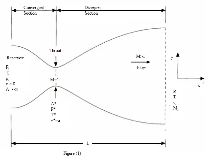
In convergent section of nozzle area is decreasing and hence velocity is increasing gradually till the throat point ,where area is such a way the Mech number is equal to zero i.e. velocity of air comes equal to speed of sound and at this point flow is called as sonic flow and, here properties like pressure and temperature are denoted by P* and T*, respectively.Flow in convergent section of nozzle before throat is subsonic i.e. flow velocity is less then speed of sound.
In the divergent section of nozzle flow expands isentropically to supersonic speed at the nozzle exit, where the exit pressure, temperature, density and mach number are denoted by Pe,Te,Ve and Me.
Here flow is 2-D but we called its 1-D because the flow properties are uniform along the axis of nozzle, it can change only in direction of flow.such flow is called as quasi 1D flow.
Control volume
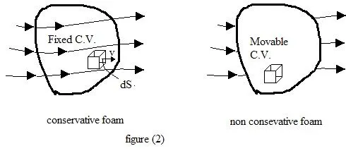
The concept of control volume when we study a flow field we consider a general flow field as represented by the imaginary lines called as streamlines and then we imagine a closed volume within a finite region this is called as controle volume.It may be fixed in space and movable.
In calssical fluid mechanicas we have approaches of study first lagrangian where we follow each and every fluid element and write flow parameter for then and second is eulerian where we study field varibles of a specifc fixed region or flow field. similar to this here we derived governing equastion of flow field in two forms in first is conservative form where the controle volume is fixed in space and fluid is moving through it or we can say fluid is crossing the surfaces those bound the controle volume and these surfaces are known as controle surfaces. second is nonconsevative form where we controle volume is moving with fluid such that fluid particales always remain inside the controle volume and now fluid partical crossing the boundary of controle volume.for the both form we derived integral (where we study a finite size CV) and differential form (where we study a infinitesimally small CV). and we derived governing equastion like
Contiuity equastion:- which is represent conservation of mass through CV
Momentum equastion:- which is represent conservation of momentum through CV
Energy equastion:- which is representconservation of energy through CV
1) Consevative form :- If we conside a fixed CV in space and apply conservation of mass through it.
then we can say mass of CV is equal to mass passing through it.
so if we say ρ is density of fluid and dV is volume of a small element of fluid inside the CV then mass of CV is
∫∫∫ρdV and time rate of increse in mass inside CV is`∂ /(∂t) ∫∫∫ρdV`
and mass passing through any controle surface as shown in figure
ρVndS =ρV.dS where S is area of surface and Vn is velocity normal to surface.
mass passing through all surfaces is
∫∫ρV.dS
so our conservation of mass equastion is
`∂ /(∂t) ∫∫∫ρdV +∫∫ρV.dS =0` ........(1)
2) Nonconsevative form :-If we conside a movable CV such that no mass cross through the boundary of CV then their only term i.e. time rate of increse in mass inside CV is`D/(Dt)∫∫∫ρdV`then our conservation of mass equastion is
`D/(Dt) ∫∫∫ρdV=0` ............(2)
here because of fluid element is moving with flow and our CV is made of infinite number of infinitesimally small elements such all is fixed inside CV or unchanginging mass inside CV, hence subtantial derivatives of these unchaningine masses equal to zerro, this is nothing but intergral form of nonconsrvative of the continuity equastion.
Let us conside a small strip in nozzle
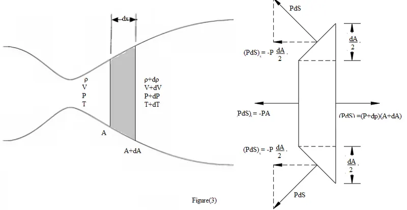
Continuity equastion :- First start with bequastion (1)
We apply this equation to a control volume which is a slice of nozzle flow, where the infinitesimal thickness of the slice is dx. Here on LHS of slice flow properties like pressure, velocity, density, and energy are denoted by P,V,𝜌 & e, respectively and they are uniform over the area A. Similarly on RHS of control volume we denote pressure, velocity, density, and energy by P+dP, V+dV, 𝜌+d𝜌 and e+de, respectively are uniform over area A+dA. In this control volume volume integral is
`∂ /(∂t) ∫∫∫_VρdV=(∂( ∂A.dx))/(∂t)`
And the surface integral term is
`∫∫_SρV.dS=ρVA+(ρ+dρ)(V+dV)(A+dA)`
Putting volume and surface integral terms in equation (1), here we get product of small entity dρ, dV and dA as these are very small so we neglect multiple of these term which is tool small.and in remaining equation when we divide by dx we get
`(∂(ρA)) /(∂t) + (∂(ρAV))/(∂x)=0`...............(3a)
`(∂ρ)/(∂t)+ ∇ .(ρV) =0` ........(3) Conservative form
Similarly
`(Dρ)/(Dt) +ρ∇ .V=0` ...........(4) Nonconservative form
Momentum equastion
Similarly we derived Momentum equastion by simply appling Newton's second law F=ma
In fulid mechnics if we consider flow is laminar,steady state, invicous and irrotational and then we apply Newton's second law and we only consider body force like gravity and pressure force normal to surface then our final momntum equastion is
`(∂ρ)/(∂t)+ρ∂z+V∂V=0`
This equastion is called euler equastion but for transient case we use only Naviour stokes equastion which include all forced due to shear,rotation and turbulence ect.and in this equastion there is also time deravitve terms
Now we turn to the integral form of the x component of momentum equation for iniviscious flow with no body forces
`∂ /(∂t) ∫∫∫_V(ρu)dV +∫∫_S(ρuV).dS =∫∫_S(PdS)_x` .........(5)
Where (P.ds)x denotes the x component of p ds and volume and space integrals are evaluated same as in continuity equation
`∂ /(∂t) ∫∫∫_V(ρu)dV=∂ /(∂t) (ρVA.dx)`
`∫∫_S(ρuV).dS=ρV^2A+(ρ+dρ)(V+dV)^2(A+dA)`
Similarly we solve it as continuity equation and we get
`(∂(ρVA))/(∂t)+(∂(ρV^2A))/(∂x) =-A(∂P)/(∂x)` ..........(6)
This is conservative form of momentum equation for obtain nonconservative form we multiplying equastion (3a) by V
`V(∂(ρA)) /(∂t) + V(∂(ρAV))/(∂x)=0`
And subtract this equation from equation (6) solving and dividing bothside by A we finally get
`ρ(∂V)/(∂t)+ρV(∂V)/(∂x) =-(∂P)/(∂x)` ...........(7)
This is nonconservative form of momentum equation
Energy equastion
Now we turn to the integral form of the energy equation for inviscious flow
`∂ /(∂t) ∫∫∫_Vρ(e+(V^2)/2)dV+∫∫_S(e+(V^2)/2)V.dS=∫∫_S(PV).dS`. ..........(8)
After solving this equastion we get Consevative form of energy equastion in terms of `e+(V^2)/2`
`(∂)/ (∂t)[ρ(e+(V^2)/2)A]+ (∂)/ (∂x)[ρ(e+(V^2)/2)VA]= − (∂(PAV))/(∂x)` .........(9)
For obtain nonconservative form, we multiplying equastion (6) by V and subtract by (9) we get
`(∂(ρeA))/ (∂t)+ (∂(ρeVA))/ (∂x)= − P (∂(AV))/(∂x)` ........(10)
This is conservative form of energy equation in terms of internal energy 'e' for quasi 1D flow for obtain nonconservative form we multiplying equastion (7) by e
`e(∂(ρA)) /(∂t) +e (∂(ρAV))/(∂x)=0`
and subtract it from eq (10)
`ρA(∂e) /(∂t) +ρAV(∂e)/(∂x)= − P (∂(AV))/(∂x)`
expand and divide by A
`ρ(∂e) /(∂t) +ρV(∂e)/(∂x)= − P (∂V)/(∂x) − PV (∂(lnA))/(∂x)` ........(11)
This is conservative form of energy equation in terms of internal energy 'e'.
e=cvT then
`ρc_v(∂T) /(∂t) +ρc_vV(∂T)/(∂x)= − P (∂V)/(∂x) − PV (∂(lnA))/(∂x)` ........(12)
now we know ideal gas equastion
P=ρRT
difrentiation wrt x we get
`(∂P)/(∂x)=R(ρ(∂T)/(∂x)+T(∂ρ)/(∂x))` .........(13)
Using above expresion we get final noncnservative form equastions
Contiuity equastion:- `(∂(ρA)) /(∂t) + ρA(∂V)/(∂x)+ρV(∂A)/(∂x)+VA(∂ρ)/(∂x)=0` ..........(14)
Momentum equastion:- `ρ(∂V)/(∂t)+ρV(∂V)/(∂x) =-R(ρ(∂T)/(∂x)+T(∂ρ)/(∂x))` ..........(15)
Energy equastion:- `ρc_v(∂T) /(∂t) +ρc_vV(∂T)/(∂x)= −ρRT [(∂V)/(∂x) +V (∂(lnA))/(∂x)]`..........(16)
Numerical solution for quasi 1D subsonic-supersonic nozzle flow :-
1) Inputs data for problem
Now for our nozzle flow broblem we have following inputs data
Area A=1+2.2*(x-1.5)2
here area of nozzle is only function of distance travel
if we conside number of grid point n=31 then dt=1
ρ=1-0.3146*x
T=-0.2314*x
V=(0.1+1.09*x)*T2
2) MacCormack's technique :- In computational fluid dynamics, the MacCormack method is a widely used discretization scheme for the numerical solution of hyperbolic partial differential equations. This second-order finite difference method was introduced by Robert W. MacCormack in 1969.The application of MacCormack method to any function f proceeds in two steps
Predictor step:- In this step first we calculate time derivative of function f useing Forward Differencing scheme for space derivative and the we calucate new value of function f which is sum of old value of and its pridictor time derivative.
I) Predictor step time derivative
`(delf)/(delt_p)=(f(i+1)-f(i))/(trianglex)`
II) Solution Update
`f'=f_(old)+(delf)/(delt_p)*trianglet`
here f' is predictor step function
`f_(old)` is initial or old value of function
`(delf)/(delt_p)` is predictor step time derivative of function
Corrector step:- In this step we calculate time derivative of function f' useing Bacward Differencing scheme for space derivative and then calculate average time derivative.
III) Corrector step time derivative
`(delf)/(delt_c)=(f(i)-f(i-1))/(trianglex)`
IV) Average time derivative
`((delf)/(delt))_(avg)=0.5**((delf)/(delt_p)+(delf)/(delt_c))`
V) Final Solution
`f'=f_(old)+((delf)/(delt))_(avg)*trianglet`
3) Appling sutable Baundary condition and calculatibg time step varibles.
Here our Flow equastions are hyperbolic in nature therefore flow in x direction exist two real characteristic lines through any point in the xy plane.These lines are labeled as left and right running characteristic Physically they represent infinitely week mach waves which are propogating upstream and downstram respectivly. and both travlling with speed of sound.
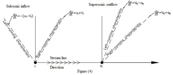
Now if we look at figure (4), there are two points i.e. 1 and N at inlet and outlet of nozzle.Flow at point 1 is subsonic i.e. flow velocity is less then speed of solund, Hence left-running characteristic at 1 is travles upstream towards left as shown in figure(4) the left-running Mach wave,which is traveling toward the left at the speed of sound easily works its way upstream against the low-velocity subsonic flow, which is slowly moving from left to right,Hence we show the left-running characteristic running to the left with a combined speed a1-V1 (relative to the fixed nozzle).Since domain is 1 to N and hence our left-running characteristic is out of domain.If one characteristic line propagates out of the domain, then the value of another dependent flow-field variable must be allowed to float at the boundary i.e., it must be calculated in steps of time as a function of the timewise solution of the flow field. then At the subonic inflow boundary, we must stipulate the values of two dependent flow-field variables, whereas the value of one other variable must be allowed to float.
if there is an internal points 2 and 3 in between the boundaries
then slope`=(V_3-V_2)/(trianglex)`
and `V_1=2**V_2-V_3`
and other values are equal to their stagnation values and fixed(independent of time).
Now at outflow boundary, located at grid point N, As before, the left-running characteristic at point N propagates to the left at the speed of sound a relative to a fluid element. However, because the speed of the fluid element itself is supersonic, the left-running characteristic is carried downstream at the speed (relative to the nozzle) ofVN-aN. The right-running characteristic at point N propagates to the right at the speed of sound a relative to the fluid element, and thus it is swept downstream at the speed (relative to the nozzle) of VN+aN.Hence, at the supersonic outflow boundary, we have both characteristics propagating out of the domain; so does the streamline at point N.Therefore, there are no flow-field variables which require their values to be stipulated at the supersonic outflow boundary.
- Solving Nonconservative form Equastions using MacCormack's technique
Step 1:- Derived Governing equastion in terms of non-dimentional varibles.
For nozzle flow , flow-field variables are frequently expressed in terms of non dimensional variables such that the flow variables are referenced to their reservoir values. The non dimensional flow variables P/P0, 𝜌/𝜌0, and T/T0 are vary between o to 1.
𝜌’=𝜌/𝜌0 and T’= T/T0
If L is length of nozzle then
x’=x/L
And a0 = speed of sound = `sqrt(gammaRT)`, then we define a dimensionless velocity as V’=V/a0
`t'=t/(L*a_0)` and A’=A/A*
Here A’ is function of x only, then
`(∂(ρ'A')) /(∂t')=A'(∂ρ') /(∂t')`
`(RT_0)/(a_(0)^2)=(gammaRT_0)/(gammaa_(0)^2)=(a_0^2)/(gammaa_0^2)=1/gamma`
`R/(c_v)=R/(R/(gamma-1))=gamma-1`
Now introducing the non dimensional variable in eq.(14),(15) and (16) and solving by using above expressions we get non-dimensional for of governing eq’s for non conservative form.
Contiuity equastion:- `(∂ρ') /(∂t')=-ρ'(∂V')/(∂x')-ρ'V'(∂(lnA'))/(∂x')-V'(∂ρ')/(∂x')` ..........(14a)
Momentum equastion:- `(∂V')/(∂t')=-V'(∂V')/(∂x') -1/gamma((∂T')/(∂x')+(T')/(ρ')(∂ρ')/(∂x'))` ..........(15a)
Energy equastion:- `(∂T') /(∂t')=-V'(∂T')/(∂x')−(gamma-1)T' [(∂V')/(∂x') +V'(∂(lnA'))/(∂x')]` ..........(16a)
Step 2:-Calculation for time steps
`△t=C(△X)/(a_0+V)` where C is CFL number and C=0.5
we calculate △t in a for loop of increment i=1 to 31
`△t=min(△t_1,△t_2,△t_3,........,△t_31)`
Step 3:-Now calculate pridictor time derivative for density ,velocity and temperature using above equastion and forward differencing scheme for space derivative.
`((∂ρ) /(∂t_p))_(j)^t=-ρ_(j)^t(V_(j+1)^t-V_j^t)/(dx)-ρ_(j)^tV_j^t(lnA_(j+1)^t-lnA_j^t)/(dx)-V_j^t(ρ_(j+1)^t-ρ_j^t)/(dx) ...............(17)`
`((∂V)/(∂t_p))_j^t=-V_j^t(V_(j+1)^t-V_j^t)/(dx) -1/gamma((T_(j+1)^t-T_j^t)/(dx)+(T_j^t)/(ρ_j^t)(ρ_(j+1)^t-ρ_j^t)/(dx)) ...............(18)`
`((∂T) /(∂t_p))_j^t=-V_j^t(T_(j+1)^t-T_j^t)/(dx)−(gamma-1)T_j^t [(V_(j+1)^t-V_j^t)/(dx) +V_j^t((lnA_(j+1)^t-lnA_j^t))/(dx)] ...............(19)`
Step 4:- Now calculated Predictor value of ρ,V and T
`rho_j^(t+trianglet)=rho_j^t+((delrho)/(delt_p))_j^t*trianglet`
`V_j^(t+trianglet)=V_j^t+((delV)/(delt_p))_j^t*trianglet`
`T_j^(t+trianglet)=T_j^t+((delT)/(delt_p))_j^t*trianglet`
Step 5:-Them calculate Corrector time derivative of ρ,V and T
`((∂ρ) /(∂t_c))_(j)^t=-ρ_(j)^(t+trianglet)(V_j^(t+trianglet)-V_(j-1)^(t+trianglet))/(dx)-ρ_(j)^(t+trianglet)V_j^(t+trianglet)(lnA_j^(t+trianglet)-lnA_(j-1)^(t+trianglet))/(dx)-V_j^(t+trianglet)(ρ_j^(t+trianglet)-ρ_(j-1)^(t+trianglet))/(dx) ...............(20)`
`((∂V)/(∂t_c))_j^t=-V_j^t(V_(j+1)^t-V_j^t)/(dx) -1/gamma((T_(j+1)^t-T_j^t)/(dx)+(T_j^t)/(ρ_j^t)(ρ_(j+1)^t-ρ_j^t)/(dx)) ...............(21)`
`((∂T) /(∂t_c))_j^(t+trianglet)=-V_j^(t+trianglet)(T_j^(t+trianglet)-T_(j-1)^(t+trianglet))/(dx)−(gamma-1)T_j^(t+trianglet) [(Vj^(t+trianglet)-V_(j-1)^(t+trianglet))/(dx) +V_j^(t+trianglet)((lnA_j^(t+trianglet)-lnA_(j-1)^(t+trianglet)))/(dx)] ...............(22)`
Step 6:-Them calculate Average time derivative of ρ,V and T
`((delrho)/(delt))_(avg)=0.5**[((delrho)/(delt_p))_j^t+((delrho)/(delt_c))_j^(t+trianglet)]`
`((delV)/(delt))_(avg)=0.5**[((delV)/(delt_p))_j^t+((delV)/(delt_c))_j^(t+trianglet)]`
`((delT)/(delt))_(avg)=0.5**[((delT)/(delt_p))_j^t+((delT)/(delt_c))_j^(t+trianglet)]`
Step 7:-Now calculated final value of flow field varibles ρ,V and T at time t+△t time step
`rho_j^(t+trianglet)=rho_j^t+((delrho)/(delt))_(ang)trianglet ........(23)`
`V_j^(t+trianglet)=V_j^t+((delV)/(delt_p))_(ang)trianglet ......(24)`
`T_j^(t+trianglet)=T_j^t+((delT)/(delt_p))_(ang)trianglet.........(25)`
Step 8:-Boundary conditions
At inlet
`rho_1=1`
`V_1=2**V_2-V_3`
`T_1=1`
At outlet
`rho_N=2**rho_((N-1))-rho_((N-2))`
`V_N=2**V_((N-1))-V_((N-2))`
`T_N=2**T_((N-1))-T_((N-2))`
Step 9:-Calculating outputs
In this step we calculated mass flow rates throught the nozzle at different time steps, we also calculates flow varibles (Like Density, Velocity,Pressure and Temperature) and Mach number at nozzle exit and throat point.
Mass flow rate `m^.=rhoA*V`
Pressure `P=rho**T`
Mach number `M=V/sqrt(T)`
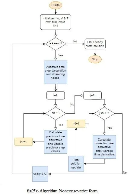
# Algorithm for Non conservative form
# Matlab function for nonconservative form
% Function for Non conservative  form
function [mass_flow_rate_NC,Pressure_NC,Mach_Number_NC,rho_NC,v_NC,T_NC,rho_NC_throat,T_NC_throat,Pressure_NC_throat,Mach_Number_NC_throat,rho_NC_exit,T_NC_exit,Pressure_NC_exit,Mach_Number_NC_exit,m_dot_NC,m_dot_NC_50ts,m_dot_NC_100ts,m_dot_NC_150ts,m_dot_NC_200ts,m_dot_NC_700ts]=fun_quasi_state_1D_nozzle_flow_Non_conservative_form(x,dx,n,gamma,nt,c)
  % Calculating Initial Condition
rho_NC=1-0.3146*x;
T_NC=1-0.2314*x;
v_NC=(0.1+1.09*x).*T_NC.^(0.5);

% Area
A=1+2.2*(x-1.5).^2;
throat=find(A==1);

% Calculating time step
for z= 1:31
    u=(T_NC(z))^(1/2);
    dt=c*dx/(u+v_NC(z));
end
dt=min(dt);

% Time Loop
for K=1:nt

  % Saving Copy of old values
  rho_old=rho_NC;
  v_old=v_NC;
  T_old=T_NC;

  % Predictor Method
  for j=2:n-1
    % Space derivative terms
    dv_dx(j)=(v_NC(j+1)-v_NC(j))/dx;
    drho_dx(j)=(rho_NC(j+1)-rho_NC(j))/dx;
    dT_dx(j)=(T_NC(j+1)-T_NC(j))/dx;
    dln_A_dx(j)=(log(A(j+1))-log(A(j)))/dx;
    % Solution
    % Continuity equastion
    drho_dt_p(j)=-rho_NC(j)*dv_dx(j)-rho_NC(j)*v_NC(j)*dln_A_dx(j)-v_NC(j)*drho_dx(j);
    % Momentum equastion
    dv_dt_p(j)=-v_NC(j)*dv_dx(j)-(1/gamma)*(dT_dx(j)+(T_NC(j)/rho_NC(j))*drho_dx(j));
    % Energy equastion
    dT_dt_p(j)=-v_NC(j)*dT_dx(j)-(gamma-1)*T_NC(j)*(dv_dx(j)+(v_NC(j)*dln_A_dx(j)));
    % Solution Update
    rho_NC(j)=rho_NC(j)+drho_dt_p(j)*dt;
    v_NC(j)=v_NC(j)+dv_dt_p(j)*dt;
    T_NC(j)=T_NC(j)+dT_dt_p(j)*dt;
  end
    % Corrector Method
  for j=2:n-1
    % Space derivative terms
    dv_dx(j)=(v_NC(j)-v_NC(j-1))/dx;
    drho_dx(j)=(rho_NC(j)-rho_NC(j-1))/dx;
    dT_dx(j)=(T_NC(j)-T_NC(j-1))/dx;
    dln_A_dx(j)=(log(A(j))-log(A(j-1)))/dx;
    % Solution
    % Continuity equastion
    drho_dt_c(j)=-rho_NC(j)*dv_dx(j)-rho_NC(j)*v_NC(j)*dln_A_dx(j)-v_NC(j)*drho_dx(j);
    % Momentum equastion
    dv_dt_c(j)=-v_NC(j)*dv_dx(j)-(1/gamma)*(dT_dx(j)+(T_NC(j)/rho_NC(j))*drho_dx(j));
    % Energy equastion
    dT_dt_c(j)=-v_NC(j)*dT_dx(j)-(gamma-1)*T_NC(j)*(dv_dx(j)+(v_NC(j)*dln_A_dx(j)));
  end
  % Average Time derivative
  drho_dt=0.5*(drho_dt_p+drho_dt_c);
  dv_dt=0.5*(dv_dt_p+dv_dt_c);
  dT_dt=0.5*(dT_dt_p+dT_dt_c);

  % Final solution Update
  for i=2:n-1
  rho_NC(i)=rho_old(i)+drho_dt(i)*dt;
  v_NC(i)=v_old(i)+dv_dt(i)*dt;
  T_NC(i)=T_old(i)+dT_dt(i)*dt;
  end
  % Appling B.C.
  % Inlet
  rho_NC(1)=1;
  v_NC(1)=2*v_NC(2)-v_NC(3);
  T_NC(1)=1;
  % Outlet
  rho_NC(n)=2*rho_NC(n-1)-rho_NC(n-2);
  v_NC(n)=2*v_NC(n-1)-v_NC(n-2);
  T_NC(n)=2*T_NC(n-1)-T_NC(n-2);

  % Getting output of function
  mass_flow_rate_NC=rho_NC.*A.*v_NC;
  Pressure_NC=rho_NC.*T_NC;
  Mach_Number_NC=v_NC./sqrt(T_NC);
  % At throat
  rho_NC_throat(K)=rho_NC(throat);
  T_NC_throat(K)=T_NC(throat);
  Pressure_NC_throat(K)=Pressure_NC(throat);
  Mach_Number_NC_throat(K)=Mach_Number_NC(throat);

  % At nozzle exit
  rho_NC_exit(K)=rho_NC(31);
  T_NC_exit(K)=T_NC(31);
  Pressure_NC_exit(K)=Pressure_NC(31);
  Mach_Number_NC_exit(K)=Mach_Number_NC(31);

  % Mass flow rate at time step 1,50,100,150,200,700
  if K==1
      m_dot_NC=mass_flow_rate_NC;
  elseif K==50
      m_dot_NC_50ts=mass_flow_rate_NC;
  elseif K==100
      m_dot_NC_100ts=mass_flow_rate_NC;
  elseif K==150
      m_dot_NC_150ts=mass_flow_rate_NC;
  elseif K==200
      m_dot_NC_200ts=mass_flow_rate_NC;
  elseif K==700
      m_dot_NC_700ts=mass_flow_rate_NC;
  end
end
end- Solving Conservative form Equastions using MacCormack's technique
Step 1:-Derived Governing equastion in terms of non-dimentional varibles.
let's start from equastion (3a)
`(∂(ρA)) /(∂t) + (∂(ρAV))/(∂x)=0`
`(∂((ρ)/(ρ_0)(A)/(A^**)))/(∂(t/(L/a_0)))((rho_0A^**a_0)/L)+ (∂((ρ)/(ρ_0)(A)/(A^**)V/a_0))/(∂x/L)((rho_0A^**a_0)/L)=0`
`(∂(ρ'A')) /(∂t') + (∂(ρ'A'V'))/(∂x')=0` ...............(14b)
This is Conservative form of continuity equastion in terms of non-dimentional varibles, for Momentum equastion we take equastion (6)
`(∂(ρVA))/(∂t)+(∂(ρV^2A))/(∂x) =-A(∂P)/(∂x)` ..........(6)
and if we expand derivative of PA
`(del(PA))/(delx)=P(delA)/(delx)+A(delP)/(delX)`. .........(26)
and put this in eq.(6)
`(∂(ρVA))/(∂t)+(∂(ρV^2A+PA))/(∂x) =P(∂A)/(∂x)`
write it in terms of non-dimentional varibles
`(∂((ρ)/(ρ_0)(V)/(a_0)(A)/(A^**)))/(∂(t/(L/a_0)))((rho_0A^**a_0^2)/L)+(∂((ρ)/(ρ_0)(V^2)/(a_0^2)(A)/(A^**)(ρ_0A^**a_0^2)+(P)/(P_0)(A)/(A^**)(P_0A^**)))/(∂(x/L)L) =P/P_0(∂A/A^**)/(∂x/L)((P_0A^**)/L)`
`(del(rho'A'V'))/(delt')+(del[rho'A'V'^2+P'A'(P_0/rho_0a_0^2)])/(delx')=P'(delA')/(delx')(P_0)/(rho_0a_0^2)`
Now we have relation
`P_0/(rho_0a_0^2)=(rho_0RT_0)/(rho_0a_0^2)=(rho_0RT_0)/(rho_0gammaRT_0)=1/gamma`
Use this in above equastion we get momentum equastion in terms of nondimentional varibles.
`(∂(ρ'V'A'))/(∂t')+(∂[ρ'V'^2A'+(1/gamma)P'A'])/(∂x') =1/gammaP'(∂A')/(∂x')` .....(15b)
Now for energy equastion we take equastion (9)
`(∂)/ (∂t)[ρ(e+(V^2)/2)A]+ (∂)/ (∂x)[ρ(e+(V^2)/2)VA]= − (∂(PAV))/(∂x)`
`(∂)/ (∂t)[ρ(e+(V^2)/2)A]+ (∂)/ (∂x)[ρ(e+(V^2)/2)VA+PAV]= 0`
write this in non diementional terms
`(∂[ρ/ρ_0(e/e_0 e_0+(V^2)/(2a_0^2)a_0^2)A/A^**])/(∂(t/(L/a_0)))((ρ_0A^**a_0)/L)+ (∂[ρ/ρ_0(e/e_0e_0+(V^2)/(2a_0^2)a_0^2)V/a_0A/A^**(ρ_0a_0A^**)+(P/P_0A/A^**V/a_0)(ρ_0a_0A^**)])/(∂(x/L)L= 0`
Since `e'=e/e_0`
`e_0=c_vT_0=(RT_0)/(gamma-1)`
`P_0/(rho_0RT_0)=(rho_0RT_0)/(rho_0RT_0)=1`
using these relation in above equastion we get
`(∂)/ (∂t')[ρ'((e')/(gamma-1)+gamma/2V'^2A']+ (∂)/ (∂x')[ρ'((e')/(gamma-1)+gamma/2V'^2)V'A'+P'A'V']= 0`. .............(16b)
This is energy equastion in terms of non-dimentional internal energy and flow varibles.
Step 2:- Derived Governing equastion in terms of Solution & flux vector and source term
Now for Numerical differencing we consider elements of the solution vector U, the flux vector F and source term J such that
`U_1=rho'A'`
`U_2=rho'A'V'`
`U_3=rho'((e')/(gamma-1)+gamma/2V'^2)A'`
`F_1=rho'A'V'`
`F_2=rho'A'V'+1/gammaP'A'`
`F_3=rho'((e')/(gamma-1)+gamma/2V'^2)V'A'+P'A'V'`
`J_2=1/gammaP'(delA')/(delx')`
here U1,U2,and U3 are dependent varibles so before time loop we calculate these initial values using initial or stagination value sof primitive varibles like density, velocity and temperature.
here `e'=e/e_0=(c_vT)/(C_vT_0)=T'`
Step 3:-Derived Pure form of flux vector
Since U1,U2, and U3 are calculated form primitive varibles, now if we calculate F1,F2,F3 and J2 with above relation it cause a problem in time marching solution, so we derived them in terms of solution vector and these are called pure form of flux vector and source term.
F1=U1. ..........(27)
`F_2=rho'A'V'+1/gammaP'A'`
`F_2=U_2^2/U_1+1/gammaU_1(gamma-1)[U_3/U_1-gamma/2(U_2/U_1)^2]`
`F_2=U_2^2/U_1+1/gamma(gamma-1)[U_3-gamma/2U_2^2/U_1]`..........(28)
and
`F_3=rho'((e')/(gamma-1)+gamma/2V'^2)V'A'+P'A'V'`. ...........(29)
`F_3=U_2(U_3/U_1-gamma/2V'^2+gamma/2V'^2)+U_2T'`. ...........(30)
`F_3=gamma(U_2U_3)/U_1-(gamma(gamma-1))/2U_2^3/U_1^2`. ...........(31)
Step 4:-Now calculate pridictor time derivative solution vector and source term
Now we use a for loop for pridictor method for j=2:n-1
first we calculate source term with forward differencing of area
`J_2=1/gammaP'(A'_(j+1)-A'_(j))/(delx')`
`J_2=1/gammarho'T'(A'_(j+1)-A'_(j))/(delx')`. ...........(32)
and then calculate time derivative of solution vector
`(delU_1)/(delt_p)=-(dF_1(j+1)-dF_1(j))/(dx) ...........(33)`
`(delU_2)/(delt_p)=-(dF_2(j+1)-dF_2(j))/(dx)+J_2 (j)...........(34)`
`(delU_3)/(delt_p)=-(dF_3(j+1)-dF_3(j))/(dx) ..........(35)`
Step 5:- Solution Update
`U_1=U_1old+(delU_1)/(delt_p)**dt ...........(36)`
`U_2=U_2old+(delU_2)/(delt_p)**dt ...........(37)`
`U_3=U_3old+(delU_3)/(delt_p)**dt ...........(38)`
here the old value are initial values
Step 6:- Update Primitive varibles
After solution update we end the for loop and decode primitive varible in terms of dependet varibles U1,U2,U3
`rho'=U_1/(A')`
`V'=U_2/U_1`
`T'=e'=(gamma-1)(U_3/U_1-gamma/2V'^2)`
Step 7:- Update Flux vector
Now use the equastions (29),(30),&(31) to update our flux vector
Step 8:-Now calculate corrector time derivative solution vector and source term
Now we use a for loop for corrector method for j=2:n-1
first we calculate source term with backward differencing of area
`J_2=1/gammarho'T'(A'_(j)-A'_(j-1))/(delx')...........(32b)`
and then calculate time derivative of solution vector
`(delU_1)/(delt_c)=-(dF_1(j)-dF_1(j-1))/(dx) ...........(33b)`
`(delU_2)/(delt_c)=-(dF_2(j)-dF(j-1))/(dx)+J_2 (j)...........(34b)`
`(delU_3)/(delt_c)=-(dF_3(j)-dF_3(j-1))/(dx) ..........(35b)`
Step 8:- Calculate Average time derivative
After ending of for loop of corrector step we calculates average time derivatives of solution vector
`((delU_1)/(delt))_(avg)=0.5**[(delU_1)/(delt_p)+(delU_1)/(delt_c)]`
`(delU_2)/(delt))_(avg)=0.5**[(delU_2)/(delt_p)+(delU_2)/(delt_c)]`
`((delU_3)/(delt))_(avg)=0.5**[(delU_3)/(delt_p)+(delU_3)/(delt_c)]`
Step 9:- Final solution update for solution vectors
Now we use a for loop for final updates
`U_1=U_1old+((delU_1)/(delt))_(avg)**dt ...........(36a)`
`U_2=U_2old+((delU_2)/(delt))_(avg)**dt ...........(37a)`
`U_3=U_3old+((delU_3)/(delt))_(avg)**dt ...........(38a)`
Step 10:- Boundary conditions
At inlet
`U_1(j=1)=(rho'A')_(j=1)`
`U_2(j=1)=2U_2(j=2)-U_2(j=3)`
`U_3(j=1)=U_1(j=1)((T')/(gamma-1)+gamma/2V'^2)`
At outlet
`(U_1)_(N)=2(U_1)_(N-1)-(U_1)_(N-2)`
`(U_2)_(N)=2(U_2)_(N-1)-(U_2)_(N-2)`
`(U_3)_(N)=2(U_3)_(N-1)-(U_3)_(N-2)`
Step 11:- Initial condition
Note :- we write initial condition before the step 2 in matlab programe
`{:(rho'=1.0),(T'=1.0):}}for 0<=x'<=0.5`
`{:(rho'=1.0-0.366(x'-0.5)),(T'=1.0-0.167(x'-0.5)):}}for 0.5<=x'<=1.5`
`{:(rho'=0.634-0.3879(x'-1.5)),(T'=0.833-0.3507(x'-1.5)):}}for 1.5<=x'<=3.5`
Step 12:- Update Primitive varibles and Calculating final outputs
`rho'=U_1/(A')`
`V'=U_2/U_1`
`T'=e'=(gamma-1)(U_3/U_1-gamma/2V'^2)`
Pressure `P=rho**T`
Mach Number `M=V/sqrtT`
mass flow rate`m^.=rhoA*V`
here we calculates density,velocity ,pressure ,Temperature and mach number at throat and exit point of nozzle.
we also calculates mass flow rate throught the nozzle at diffrent time steps.
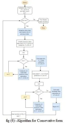
# Algorithm for Conservative form
# Matlab function for Conservative form
% Function for Non conservative  form
function [mass_flow_rate_C,Pressure_C,Mach_Number_C,rho_C,v_C,T_C,rho_C_throat,T_C_throat,Pressure_C_throat,Mach_Number_C_throat,rho_C_exit,T_C_exit,Pressure_C_exit,Mach_Number_C_exit,U1,U2,U3,m_dot_C,m_dot_C_50ts,m_dot_C_100ts,m_dot_C_150ts,m_dot_C_200ts,m_dot_C_700ts]=fun_quasi_state_1D_nozzle_flow_conservative_form(x,dx,n,gamma,nt,c)
 % Calculating Initial Condition
 % Area
A=1+2.2*(x-1.5).^2;
throat=find(A==1);

% Density and Temperature
 for i= 1:length(x)
    if x(i)>=0 && x(i)<=0.5
        rho_C(i) = 1;
        T_C(i)= 1;
    elseif x(i)>=0.5 && x(i)<=1.5
        rho_C(i) = 1.0-0.366*(x(i)-0.5);
        T_C(i) =1.0-0.167*(x(i)-0.5);
    elseif x(i)>=1.5 && x(i)<=3.5
        rho_C(i) = 0.634-0.3879*(x(i)-1.5);
        T_C(i) = 0.833-0.3507*(x(i)-1.5);
    end
 end

% Velocity
v_C = 0.59./(rho_C.*A);

% Calculating solution terms
U1=rho_C.*A;
U2=rho_C.*A.*v_C;
U3=rho_C.*A.*((T_C./(gamma-1))+(gamma/2).*v_C.^2);

 % Time steps controle
for z= 1:31
    u=(T_C(z))^(1/2);
    dt=c*dx/(u+v_C(z));
end
dt=min(dt);

% Time Loop
for K=1:nt

  % Storing initial Solustion terms
  U1old=U1;
  U2old=U2;
  U3old=U3;

  % calculating flux terms
  F1=U2;
  F2=((U2.^2)./U1)+((gamma-1)/gamma)*(U3-((gamma/2)*(U2.^2)./U1));
  F3=((gamma*U2.*U3)./U1)-((gamma*(gamma-1)/2)*(U2.^3)./(U1.^2));
  % Predictor Method
  for j=2:n-1
    % Computing source term and Space derivative terms
    J2(j) = (1/gamma)*rho_C(j)*T_C(j)*((A(j+1)-A(j))/dx);
    dU1_dt_P(j)=-(F1(j+1)-F1(j))/dx;
    dU2_dt_P(j)=(-(F2(j+1)-F2(j))/dx)+J2(j);
    dU3_dt_P(j)=-(F3(j+1)-F3(j))/dx;
    % Solution Update
    U1(j)=U1(j)+dU1_dt_P(j)*dt;
    U2(j)=U2(j)+dU2_dt_P(j)*dt;
    U3(j)=U3(j)+dU3_dt_P(j)*dt;
  end

   % Updated values
   rho_C=U1./A;
   v_C=U2./U1;
   T_C= (gamma-1)*((U3./U1)-(gamma/2)*v_C.^2);
   % Updating flux values
   F1=U2;
   F2=(U2.^2./U1)+((gamma-1)/gamma)*(U3-((gamma/2)*(U2.^2)./U1));
   F3=((gamma*U2.*U3)./U1)-((gamma*(gamma-1)/2)*(U2.^3)./(U1.^2));

  % Corrector Method
    for j= 2:n-1
      % Computing source term and Space derivative terms
      J2(j) = (1/gamma)*rho_C(j)*T_C(j)*((A(j)-A(j-1))/dx);
      dU1_dt_C(j)=-(F1(j)-F1(j-1))/dx;
      dU2_dt_C(j)=(-(F2(j)-F2(j-1))/dx)+J2(j);
      dU3_dt_C(j)=-(F3(j)-F3(j-1))/dx;
    end

     % Average Time derivative
     dU1_dt=0.5.*(dU1_dt_P+dU1_dt_C);
     dU2_dt=0.5.*(dU2_dt_P+dU2_dt_C);
     dU3_dt=0.5.*(dU3_dt_P+dU3_dt_C);

     % Final solution Update
      for w=2:n-1
          U1(w)=U1old(w)+dU1_dt(w)*dt;
          U2(w)=U2old(w)+dU2_dt(w)*dt;
          U3(w)=U3old(w)+dU3_dt(w)*dt;
      end

  % Appling B.C.
  % Inlet
  U1(1)=rho_C(1).*A(1);
  U2(1)=2*U2(2)-U2(3);
  U3(1)=U1(1)*((T_C(1)/(gamma-1))+(gamma/2)*v_C(1).^2);

  % Outlet
  U1(n)=2*U1(n-1)-U1(n-2);
  U2(n)=2*U2(n-1)-U2(n-2);
  U3(n)=2*U3(n-1)-U3(n-2);

  % Calcultaing primitive variables
  rho_C=U1./A;
  v_C=U2./U1;
  T_C= (gamma-1)*((U3./U1)-(gamma/2)*v_C.^2);

  % Getting output of function
  mass_flow_rate_C=rho_C.*A.*v_C;
  Pressure_C=rho_C.*T_C;
  Mach_Number_C=v_C./sqrt(T_C);

  % At throat
  rho_C_throat(K)=rho_C(throat);
  T_C_throat(K)=T_C(throat);
  Pressure_C_throat(K)=Pressure_C(throat);
  Mach_Number_C_throat(K)=Mach_Number_C(throat);

  % At nozzle exit
  rho_C_exit(K)=rho_C(31);
  T_C_exit(K)=T_C(31);
  Pressure_C_exit(K)=Pressure_C(31);
  Mach_Number_C_exit(K)=Mach_Number_C(31);

    % Mass flow rate at time step 1,50,100,150,200,700
  if K==1
      m_dot_C=mass_flow_rate_C;
  elseif K==50
      m_dot_C_50ts=mass_flow_rate_C;
  elseif K==100
      m_dot_C_100ts=mass_flow_rate_C;
  elseif K==150
      m_dot_C_150ts=mass_flow_rate_C;
  elseif K==200
      m_dot_C_200ts=mass_flow_rate_C;
  elseif K==700
      m_dot_C_700ts=mass_flow_rate_C;
  end
end
end- Main program that call conservative and nonconservative form functions and plots the desire output graph
%SOLVING QUASI 1D NOZZLE FLOW EQUATIONS
clear all
close all
clc

% INPUT PARAMETERS
% No. of grid points
n = 31;
gamma = 1.4;
x = linspace(0,3,n);
dx = x(2) - x(1);

%No. of time step
nt = 1400;
time_steps=linspace(1,nt,nt);

%Courant Number or CFL number
c= 0.5;


% Calling function for Non-conservative form
tic
[mass_flow_rate_NC,Pressure_NC,Mach_Number_NC,rho_NC,v_NC,T_NC,rho_NC_throat,T_NC_throat,Pressure_NC_throat,Mach_Number_NC_throat,rho_NC_exit,T_NC_exit,Pressure_NC_exit,Mach_Number_NC_exit,m_dot_NC,m_dot_NC_50ts,m_dot_NC_100ts,m_dot_NC_150ts,m_dot_NC_200ts,m_dot_NC_700ts]=fun_quasi_state_1D_nozzle_flow_Non_conservative_form(x,dx,n,gamma,nt,c);
Time_NC=toc

% Calling function for Conservative form
tic
[mass_flow_rate_C,Pressure_C,Mach_Number_C,rho_C,v_C,T_C,rho_C_throat,T_C_throat,Pressure_C_throat,Mach_Number_C_throat,rho_C_exit,T_C_exit,Pressure_C_exit,Mach_Number_C_exit,U1,U2,U3,m_dot_C,m_dot_C_50ts,m_dot_C_100ts,m_dot_C_150ts,m_dot_C_200ts,m_dot_C_700ts]=fun_quasi_state_1D_nozzle_flow_conservative_form(x,dx,n,gamma,nt,c);
Time_C=toc

% Plotting results
% Non conservative form
% Steady-state distribution of primitive variables inside the nozzle
   figure (1)
  subplot(4,1,1)
  plot(x,Mach_Number_NC)
  hold on
  plot([0 x(16)],[Mach_Number_NC(16) Mach_Number_NC(16)],'--','color','k')
  hold on
  plot([x(16) x(16)],[0 Mach_Number_NC(16)],'--','color','k')
  hold on
  plot([0 x(30)],[Mach_Number_NC(31) Mach_Number_NC(31)],'--','color','k')
  yticks([1 Mach_Number_NC(31)]);
  yticklabels({Mach_Number_NC(16),Mach_Number_NC(31)})
  title('Varition of Properties wrt Distance for Nonconservative form at 1400 Time step')
  grid on
  ylabel('Mach Number')

  subplot(4,1,2)
  plot(x,Pressure_NC)
  hold on
  plot([0 x(16)],[Pressure_NC(16) Pressure_NC(16)],'--','color','k')
  hold on
  plot([x(16) x(16)],[0 Pressure_NC(16)],'--','color','k')
  hold on
  plot([0 x(31)],[Pressure_NC(31) Pressure_NC(31)],'--','color','k')
  yticks([Pressure_NC(31) Pressure_NC(16) 1]);
  yticklabels({Pressure_NC(31),Pressure_NC(16),'1'})
  grid on
  ylabel('Presure ratio')

  subplot(4,1,3)
  plot(x,rho_NC)
  hold on
  plot([0 x(16)],[rho_NC(16) rho_NC(16)],'--','color','k')
  hold on
  plot([x(16) x(16)],[0 rho_NC(16)],'--','color','k')
  hold on
  plot([0 x(31)],[rho_NC(31) rho_NC(31)],'--','color','k')
  yticks([rho_NC(31) rho_NC(16) 1]);
  yticklabels({rho_NC(31),rho_NC(16),'1'})
  grid on
  ylabel('Dendity ratio')

  subplot(4,1,4)
  plot(x,T_NC)
  hold on
  plot([0 x(16)],[T_NC(16) T_NC(16)],'--','color','k')
  hold on
  plot([x(16) x(16)],[0 T_NC(16)],'--','color','k')
  hold on
  plot([0 x(31)],[T_NC(31) T_NC(31)],'--','color','k')
  yticks([T_NC(31) T_NC(16) 1]);
  yticklabels({T_NC(31),T_NC(16),'1'})
  grid on
  xlabel('X')
  ylabel('Temperature ratio')

% Time-wise variation of the primitive variables at throat and exit point
  figure(2)
  subplot(4,2,1)
  plot(time_steps,Mach_Number_NC_throat)
  title('Varition of properties wrt Time step for Nonconservative form at throat')
  grid on
  ylabel('Mach Number')

  subplot(4,2,2)
  plot(time_steps,Mach_Number_NC_exit)
  title('Varition of properties wrt Time step for Nonconservative form exit of nozzle')
  grid on
  ylabel('Mach Number')

  subplot(4,2,3)
  plot(time_steps,Pressure_NC_throat)
  grid on
  ylabel('Pressure ratio')
  subplot(4,2,4)
  plot(time_steps,Pressure_NC_exit)
  grid on
  ylabel('Pressure ratio')

  subplot(4,2,5)
  plot(time_steps,rho_NC_throat)
  grid on
  ylabel('Dendity ratio')
  subplot(4,2,6)
  plot(time_steps,rho_NC_exit)
  grid on
  ylabel('Dendity ratio')

  subplot(4,2,7)
  plot(time_steps,T_NC_exit)
  grid on
  xlabel('Time Steps')
  ylabel('Temperature ratio')
  subplot(4,2,8)
  plot(time_steps,T_NC_exit)
  grid on
  xlabel('Time Steps')
  ylabel('Temperature ratio')

  % Variation of Mass flow rate distribution inside the nozzle at different time steps
  figure(3)
  plot(x,m_dot_NC,'color','b')
  hold on
  plot(x,m_dot_NC_50ts,'color','g')
  plot(x,m_dot_NC_100ts,'color','m')
  plot(x,m_dot_NC_150ts,'color','y')
  plot(x,m_dot_NC_200ts,'color','r')
  plot(x,m_dot_NC_700ts,'color','y')
  plot(x,mass_flow_rate_NC,'color','K')
  title('Mass flow rate distribution for Nonconservative form through the nozzle at different time steps')
  legend('1st Time step','50th Time step','100th Time step','150th Time step','200th Time step','700th Time step','1400th Time step')
  xlabel('x')
  ylabel('Mass flow rate')


  % Conservative form
  % Steady-state distribution of primitive variables inside the nozzle
  figure (4)
  subplot(4,1,1)
  plot(x,Mach_Number_C)
  hold on
  plot([0 x(16)],[Mach_Number_C(16) Mach_Number_C(16)],'--','color','k')
  hold on
  plot([x(16) x(16)],[0 Mach_Number_C(16)],'--','color','k')
  hold on
  plot([0 x(30)],[Mach_Number_C(31) Mach_Number_C(31)],'--','color','k')
  yticks([1 Mach_Number_C(31)]);
  yticklabels({Mach_Number_C(16),Mach_Number_C(31)})
  title('Varition of Properties wrt Distance for Conservative form at 1400 Time step')
  grid on
  ylabel('Mach Number')

  subplot(4,1,2)
  plot(x,Pressure_C)
  hold on
  plot([0 x(16)],[Pressure_C(16) Pressure_C(16)],'--','color','k')
  hold on
  plot([x(16) x(16)],[0 Pressure_C(16)],'--','color','k')
  hold on
  plot([0 x(31)],[Pressure_C(31) Pressure_C(31)],'--','color','k')
  yticks([Pressure_C(31) Pressure_C(16) 1]);
  yticklabels({Pressure_C(31),Pressure_C(16),'1'})
  grid on
  ylabel('Presure ratio')

  subplot(4,1,3)
  plot(x,rho_C)
  hold on
  plot([0 x(16)],[rho_C(16) rho_C(16)],'--','color','k')
  hold on
  plot([x(16) x(16)],[0 rho_C(16)],'--','color','k')
  hold on
  plot([0 x(31)],[rho_C(31) rho_C(31)],'--','color','k')
  yticks([rho_C(31) rho_C(16) 1]);
  yticklabels({rho_C(31),rho_C(16),'1'})
  grid on
  ylabel('Dendity ratio')

  subplot(4,1,4)
  plot(x,T_C)
  hold on
  plot([0 x(16)],[T_C(16) T_C(16)],'--','color','k')
  hold on
  plot([x(16) x(16)],[0 T_C(16)],'--','color','k')
  hold on
  plot([0 x(31)],[T_C(31) T_C(31)],'--','color','k')
  yticks([T_C(31) T_C(16) 1]);
  yticklabels({T_C(31),T_C(16),'1'})
  grid on
  xlabel('X')
  ylabel('Temperature ratio')

  % Time-wise variation of the primitive variables at throat and exit point
  figure(5)
  subplot(4,2,1)
  plot(time_steps,Mach_Number_C_throat)
  title('Varition of properties wrt Time step for Conservative form at throat')
  grid on
  ylabel('Mach Number')
  subplot(4,2,2)
  plot(time_steps,Mach_Number_C_exit)
  title('Varition of properties wrt Time step for Conservative form at nozzle exit')
  grid on
  ylabel('Mach Number')

  subplot(4,2,3)
  plot(time_steps,Pressure_C_throat)
  grid on
  ylabel('Pressure ratio')
  subplot(4,2,4)
  plot(time_steps,Pressure_C_exit)
  grid on
  ylabel('Pressure ratio')

  subplot(4,2,5)
  plot(time_steps,rho_C_throat)
  grid on
  ylabel('Dendity ratio')
  subplot(4,2,6)
  plot(time_steps,rho_C_exit)
  grid on
  ylabel('Dendity ratio')

  subplot(4,2,7)
  plot(time_steps,T_C_throat)
  grid on
  xlabel('Time Steps')
  ylabel('Temperature ratio')
  subplot(4,2,8)
  plot(time_steps,T_C_exit)
  grid on
  xlabel('Time Steps')
  ylabel('Temperature ratio')

  % Variation of Mass flow rate distribution inside the nozzle at different time steps
  figure(6)
  plot(x,m_dot_C,'color','b')
  hold on
  plot(x,m_dot_C_50ts,'color','g')
  plot(x,m_dot_C_100ts,'color','m')
  plot(x,m_dot_C_150ts,'color','y')
  plot(x,m_dot_C_200ts,'color','r')
  plot(x,m_dot_C_700ts,'color','y')
  plot(x,mass_flow_rate_C,'color','K')
  title('Mass flow rate distribution for conservative form through the nozzle at different time steps')
  legend('1st Time step','50th Time step','100th Time step','150th Time step','200th Time step','700th Time step','1400th Time step')
  xlabel('x')
  ylabel('Mass flow rate')
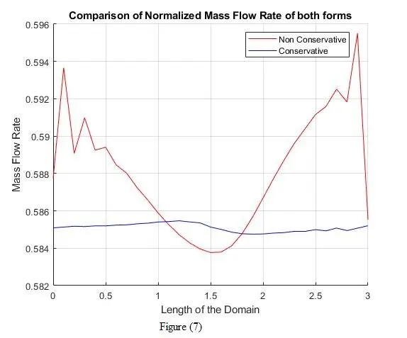
%COMPARISON PLOT of Normalized Mass Flow Rate of both forms
figure(7)
hold on
plot(x,mass_flow_rate_NC,'r')
hold on;
plot(x,mass_flow_rate_C,'b')
hold on;
grid on
legend('Non Conservative','Conservative');
xlabel('Length of the Domain')
ylabel('Mass Flow Rate')
title('Comparison of Normalized Mass Flow Rate of both forms')Results:-
Time_NC =
0.0917
Time_C =
0.1259
From the above result it is clear that time elapse to run function of numconservative form is less then time elapse to run function of conservative form.This because numconservative form function there no need to decoding the primitive varible to flux varible so it take less effrot to exicute the function.
# As per give in the problem we have to plot
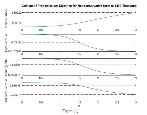
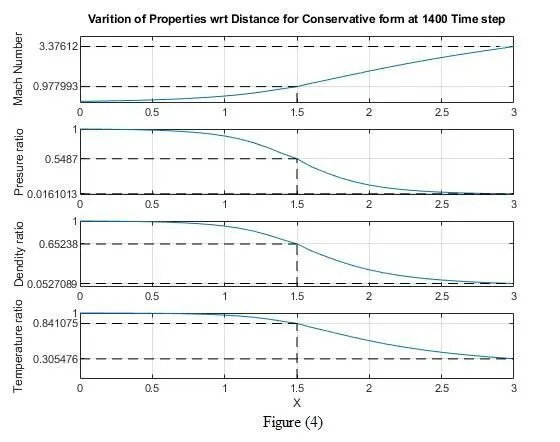
1. Steady-state distribution of primitive variables inside the nozzle
In the main program, When we plot flow variables like mach number , Pressure ratio, density ratio and temperature ratio with respect to x for both Nonconservative and conservative forms in figure 1 and figure 4 we get nearly simillar results in both plots, where mach number is intially less then 1 ( i.e. subsonic flow )and increasing with positive slope upto 1 (i.e. sonic flow) at throat point then increase with negative slope until the nozzle exit (i.e. flow at exit is supersonic).This patterns are shown in both the plots.
If we look at Pressure, Density and temperatue plots in fig 1 & 4, we observed initially these values are equal to 1 and decreasing with positive slope till the throat point and the further more decreasing with negative slope until the nozzle exit.here only diffrence is pressure decrease more rapidly as compare to density and temperature in subsonic flow where in supersonic flow pressure ,density and temperature all decrease in normal way upto a certain non zero value.
2. Time-wise variation of the primitive variables
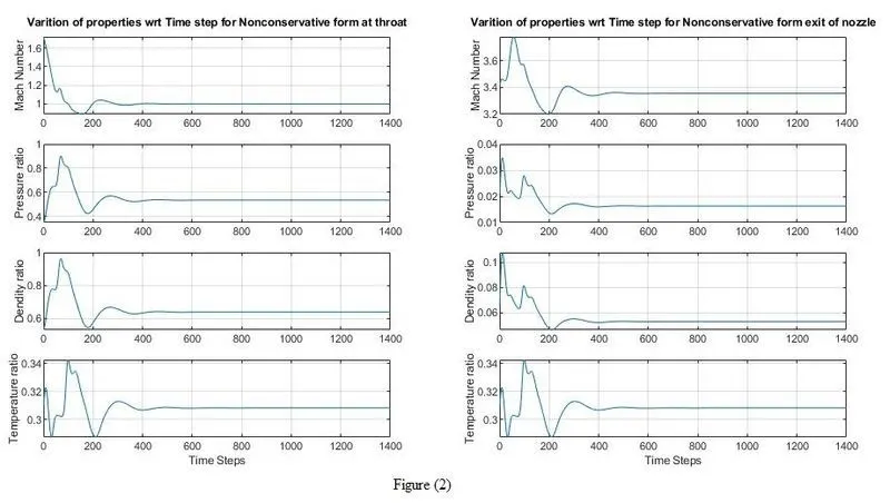
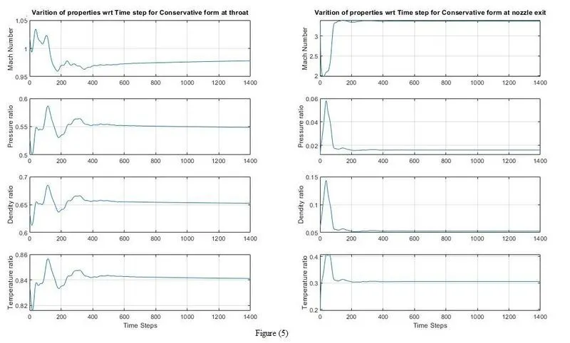
Here in above figures, you may noted that at throat point Mach number is not equal to 1 ( in analytical solution mach number at throat is 1,i.e. sonic flow) however in both form its value is not exactly equalt 1 but approximate near to 1. Like this values of pressure, density and temperrature also different in both the forms. In the time marching solution the values these flow varibles change from current time step to the next time step.
When we plot a graph betweent all the flow varibles at troat and nozzle exit, with respect to time step you can easily observed that at initial time step values of not near to its accurate values. If we look at mach number varition at throat initial its value is 1.6 in nonconservative form and when we increase time steps it is rapidy decrease and slightly around 200 time steps and then comes nearly equalt to 1 after 500 time steps.and in conservative form its varition is not similar to the nonconservative form and it take more 1000 time step to reach at approximate value so we acn say that conservative form takes more time steps to get approximate values of flow varibles. But if observe in graphs at nozzle exit both the form takes nearly 400 to 500 time steps to reach at final approximate values of flow varibles.
3. Variation of Mass flow rate distribution inside the nozzle at different time steps during the time-marching process
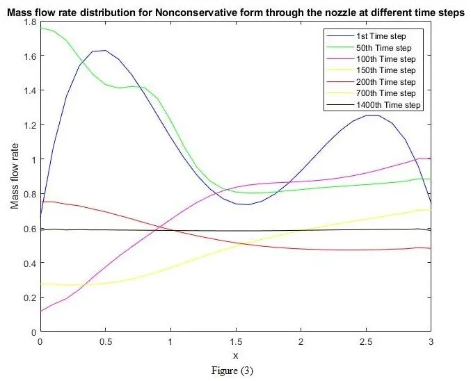
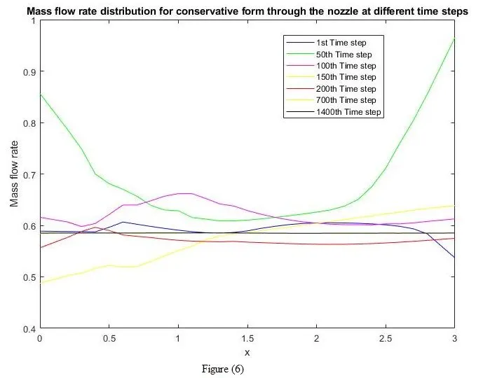
Now look at bellow graphes at time step '1 ' mass flow rate varition through out nozzle by 'blue' colour plot and we observe here in conservative it varies less and in nonconservative form it varies up to 2.5 times and at exit come to initial value.And at time '50' grean colour graph in consevative form initially it is high but at throat point it move constantly and suddenly go to high value but in nonconsrvative form initially it is high befor the throat and moves nearly at constant value.Similary if we observe 100 time step 'magenta' colour plot it is also diffrent in both forms.And if ypu notice plots for time steps 150,200,700 and 1400 are nearly same for both the forms.
So for higher time step mass flow rate distribution inside the nozzle are nearly similar in both conservative and nonconservative foms.And as time steps increases mass flow rate distribution inside the nozzle became constant.
4. Comparison of Normalized mass flow rate distributions of both forms
Now if we plot mass flow rate at final time step for both the forms in a single figure (7).You may observed that conservative form does a better job of preserving mass flow rate throughout the flow field and it is mainly because the mass flow rates itself is one of dependent varible in equastion where in noncoservative form only primitive varibles (rho, V and T) are dependent varibles and mass flow rate is secondary result.
Conclusion:-
- The Conservative form yields a better mass flow distribustion as compare to nonconservative form. The conservative form simply does a better job of conserving mass.
- In steady state calculation of primitive varible (like density, velocity, temperature, pressure and mach number) noncoservative form give slightly more accurate result then coservative form.
- In transient calculation of primitive varible noncoservative form converge in slightly less time steps as compare to coservative form.
- Noncoservative form takes less time to execute the programe as compare to coservative form.