Project 2 - Rankine cycle Simulator
Aim:- Aim of this project to simulate rankine cycle in matlab using steam data and plot T-s and h-s diagram.
Theory:- A Rankine cycle is an "Vapour Power Ideal Thermodyanamic Cycle" on which steam power plant's are working. It is first introduce by scottish engineer 'William J.M. Rankine' in 1859.
This cycle is a practical example of carnot cycle but it is not exactly carnot cycle but it similar to it.
Carnot cycle is an " Reversible Ideal Thermodynamic Cycle" operate with gas or vapour both. It was first introduce in 1824 by a franch physicist 'Nicolos Leonard Said Carnot' in his monogram name "Reflection of Motive Power of Fire" where carnot explain how we can produce work from energy produce by heating or burning fule.
In this carnot explain varius thermodynamic process like Isochoric(Volume constant), Isobaric(Pressure Costant), Isothermal(Tempereture constant), Adiabetic and polytropic with heat transfer and work tranfer. And Also explain a cycle ' A complete loop of varius process (compression, heating expansion and cooling) in such a way initial and last point are same. These cycle are either power producing device (heat engine) or power absorbing device (heat pump or refgerator).
All power producing cycle are clockwise on P-V, T-S and H-S digram and all power absorbing cycle are anticlockwise.
In this carnot give an principle which sate that
1. Revesible cycle efficency is always grater then all irrevesibe cycle operate between same thermal energey reservoir i.e. source (TH) and Sink (TL).
2. Efficieny of reversible cycle is independent of working fluid and it is function of thermprature limits only.
Now here Reversible term is use for both either process and cycle.
Rversible proces:- It is a process which follow same path when we revese it that means there no energy losser due to friction, randomness and other dissipative effects.
A total reversible cycle is reversible either internaly (i.e. No entropy generation inside the system) or externaly (i.e. no change in entropy).
Entropy is a propery of the system and it not depend on path it is a point function. Physiscaly it is represent randomness of the system or randomness of the micro particales (atoms) of the system. When a system have heigher entropy then probability of loss of energy is more at this state because randomness of parical is more.
Entropy change is a path function and it represent loss of energy during the process.
`ds = (delQ)/T +dels _(Gen)`
The process like Heating , cooling , compression and expansion have no heat generation we called them internal reversible but if say a process have no change in entropy we say them isentropic.
but the process which have bith no heat generation and no change in entropy we called them total revesible process. In Adiabetic process have no heat transfer and when it is reversible (i.e. no heat generation) then change is entropy ds=0.
This is called as Reversible Adiabetic Process (because sgen=0 and Q=0) or Isentropic (because ds=0). All Reversible Adiabetic Process are Isentropic but all Isentropic process are not need to be either reversibe or adiabetic. Irreversible cooling with sgen= dQ/T is isentropic (because ds = 0)
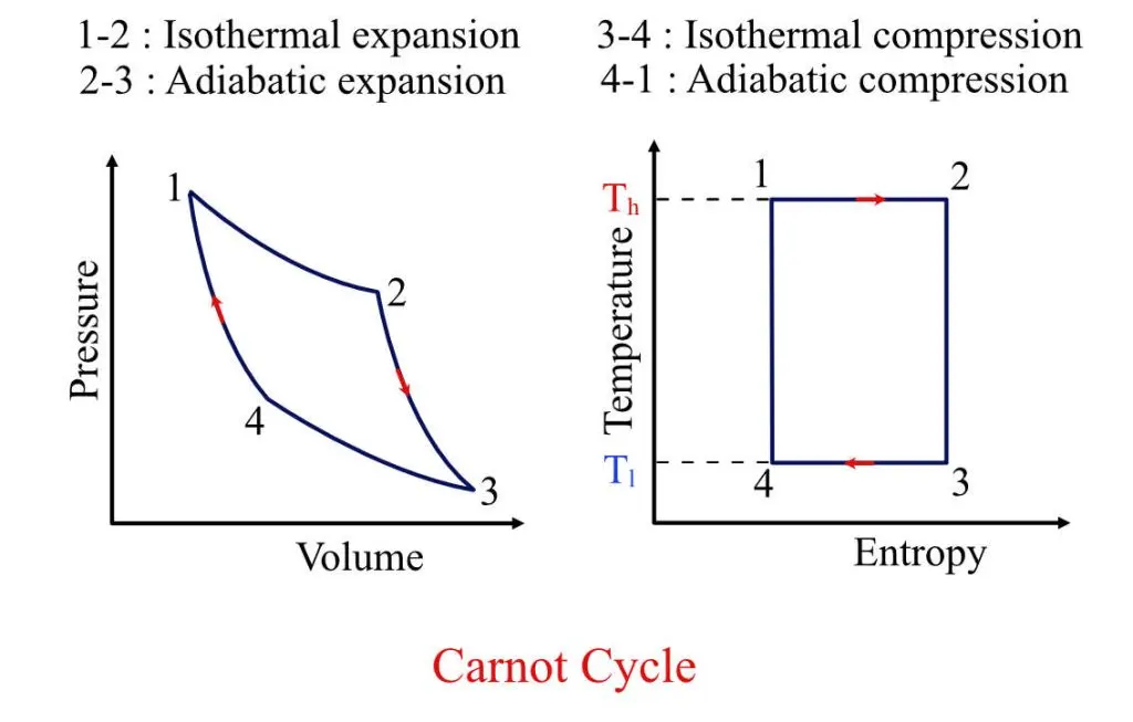
This cycle contain four process out of which two are Isentropic compression and expansion. And remaining two are Isothermal Heating and Cooling. These process are completely itheoritical because in real case process like compresion and expantion have some amount of entropy generation which thens to increase entropy of system.
Isothermal Heating and cooling is not possible for a single phase substance like gas but if we use vapour which may be liquid and gas states. Because during phase change themperature is not change.
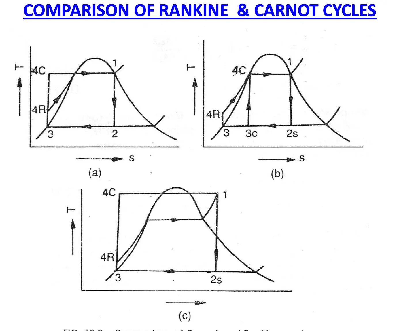
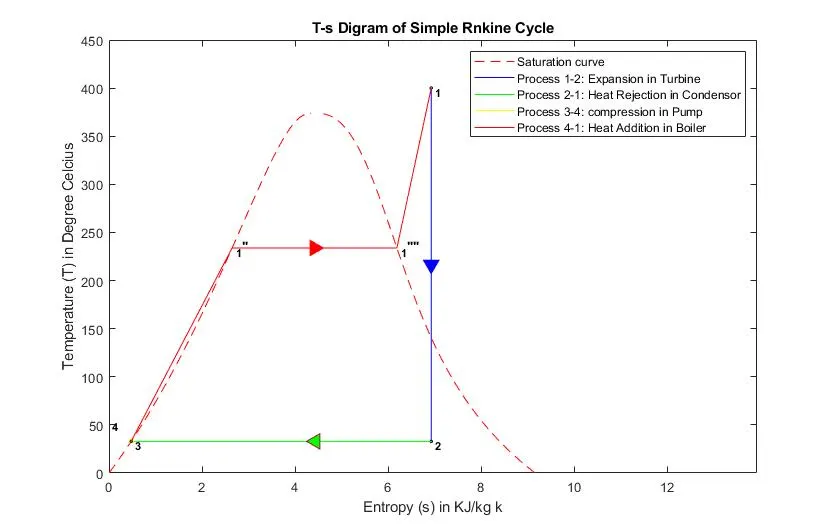
Here in above T-s plots you may see a dome cureve called as Saturation curve the RHS region of this curve is gass phase region (i.e. steam exitance) and LHS region is liquid region (i.e.water exitance of water). Mid region is called as wet region a mixer of liquid and gas.
When we heat water at constant pressure (Isobaric process) it tempreature is increasing untill the saturated liquid point here water start to change into vapour and as we give heat to it's tmeperature not changine it's convert to its latent heat (L.H.) till the saturated gas or vapour point here it completely convert into steam and if we gave more heat it temperature is again increasing and stemp called super heated steam.
A Rankine cycle is an modified version of carnot cycle with working fluid as vapour.It is not a reversibele cycle but efficency is nearly to the carnot cycle.
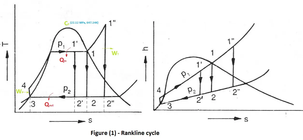
Process 1-2 : Isentropic Expansion in Turbine
Here three condition of Rnakine cycle is possible for turbine as shown in above figure
1 Inlet is at Saturated curve
1' Inlet is at Wet region
1" Inlet is at superheated region (Mean Temperature of heat addtion is increase)
Process 2-3 : Isobaric Heat Rejection in Condesor
Again 3 condtions are thre point 2 is either on the Saturated curve, in side wet region and at superheated region
In this project our study is on two case
1. Turbine inlet is super heated and condesor inlet is in wet region
2. Turbine inlet is super heated and condesor inlet is in super heated region (Mean Temperature of heat Rejection is high)
Process 3-4 : Isentropic comprasion in Pump
Process 1-2 : Isobaric Heat Addirion in Boiler
Varition of Rankine cycle
1. Superheated Rankine Cycle (our study is on this)
In this cycle efficiency increase because Turbine work increase, Net work increase more because mean temperature of heat addtion increase so area under curve 4-1 on T-s diagram increase so ammount of heat addition in boiler also increase.
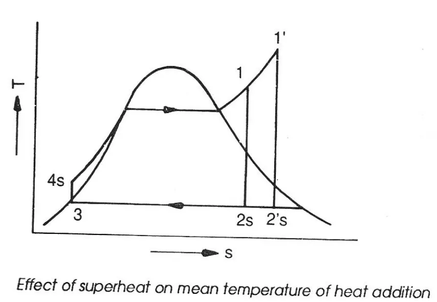
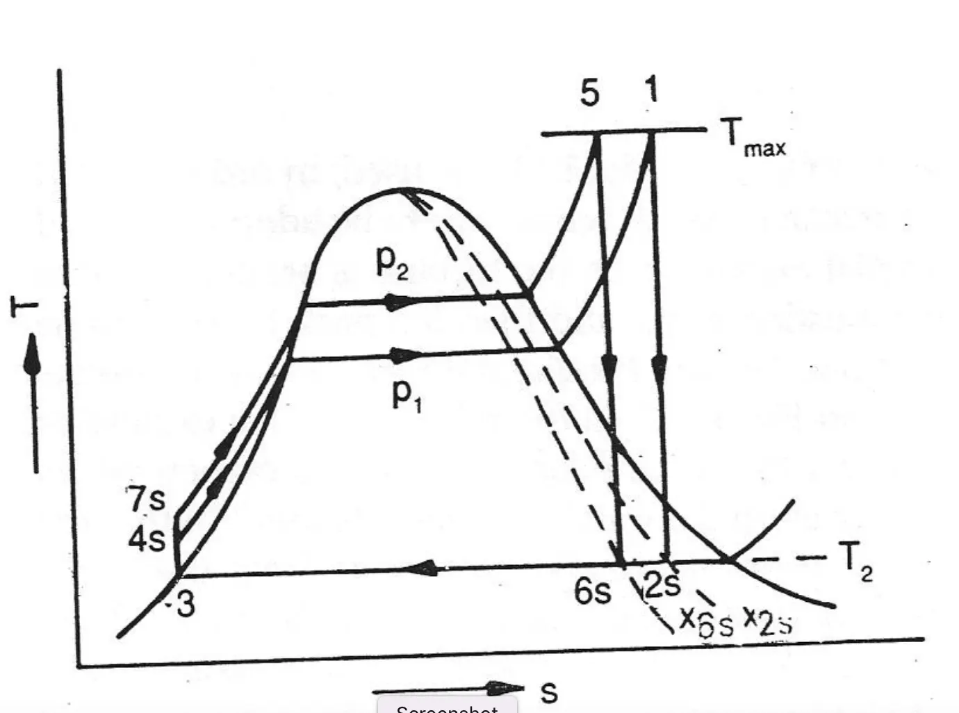
Limitation metrological of temperature for turbine blades so we need to increase pressure of boiler to increase mean tempreature of heat addition to get max work.
2. Reheated Rankine Cycle
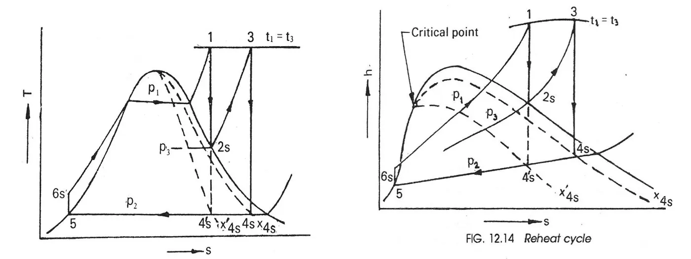
Turbine work ioncrease WT1=h1-h2s and WT2=h3-h4s and WT=h1+h3-(h2+h4) which is more then a single turbine work in superheted cycle.
Here we dont need to increase pr. of boiler to get max work.
Limitation Reheat shoild be on Optimum pressure so intial cost is high.
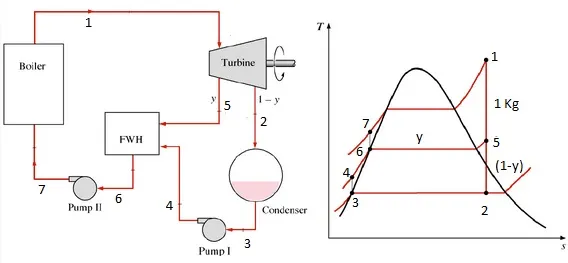
3. Regenerated rankine cycle
# Matlab code to plot these cycle T-s and H-s daiagram.
There is an standereded steam table is use to findout enthalpy,entropy, specific volume, specific heat at different Temperature and pressure , saturation curve and crtical point etc.
There is a Function script XSteam.m for matalb which returns these thermodanamic properies.
1. To get enthalpy h in KJ/Kg at pressure p bar and temperature T in degree celcius
h1=XSteam('h_pT',p1,T1)
2. To get enthalpy h in KJ/Kg at pressure p bar on saturate curve
hf1=XSteam('hL_p',p1) for saturated liquid curve
hv1=XSteam('hV_p',p1) for saturated vapour curve
3. Simlarly for enthalpy s in KJ/Kg degree celcius
s1=XSteam('s_pT',p1,T1)
sf1=XSteam('sL_p',p1) for saturated liquid curve
sv1=XSteam('sV_p',p1) for saturated vapour curve
4. Cp in kJ/kg degree celcius
cpl1=XSteam('cpL_p',p1) for saturated liquid curve
cpv1=XSteam('cpV_p',p1) for saturated vapour curve
Now write the programe with input data given in problem statement
Case 1
p1=30 bar
P2 = 0.05 bar
T1 = 400 degree celcuis
Case 2
p1=44 bar
P2 = 5.83 bar
T1 = 538 degree celcuis
1. Frist print all process names on workspac using fprintf
2. Input these data on varible p1,p2 and T1
3. Calcualte Temperature, enthalpy and entropy at each state point useing above code and print them on workspace.
a. on state 1 we have given p1 and T1 we directly get s1 and h1 using above code.
b. on state 2 we have two case first point 2 in side the wet region and second point 2 on superheated region
so first we calcualted dryness fraction (ration of mass of vapour to total mass of substance at point)
x=(sg-s)/(sg-sf)
so first we calcualte sg and sf at p2 and we know process 1-2 is isentropic i.e. s2=s1, using these data we calcualte x2 if it is less then equal to 1 i.e., point 2 in wet region (case1) else pont 2 in superheated region (case2).
Now using contional statement ffor x<=1 (in wet region we calcualted h by formula
h=hf+x*(hg-hf)
else
h=hg+CpV*(T2-Tsat_p2)
T2 is calcualte at s2 and p2 by using XSteam.m data
and Tsat_p2 is Saturated temperatre at pressure p2 calcualte using XSteam.m data
c. on State 3 we say consdesor pressure and temperature is constant and get s3=sf2 and h3=hf2.
d. On state 4 we consider s4=s3 and p4=p1 and get T4 = Xsteam('T_ps',p4,s4) and h4=XSteam('h_pT',p4,T4)
4. Now calcualte
a. carnot efficieny
b. Rankine cycle efficency
c. Net work output
d. back work ratio
e. specific fuel consuption
5. Now for Plotting T-s and h-s diagram.
a firts crate a lineare space ofr temperature 0 to 1000 having 4000 indexs
b. now using for loop create staurate liquid and vapour curves varible for each value of temperatre on T-s and h-s curve.
c. Now first plot T-s digaram in figure(1)
plot Saturation curve , linetype dash and color red.
hold on
Then plot each state point as a marker 'o' and using text commond name it.
plot each process with arrow using marker '>','<','^'&'V' with diffrent color
d. give title, legend and labeles and hold off
e. using above steps plot h-s diagram.
%% Matlab code for Rankine Cycle Simulator
close all
clear all
clc

fprintf('\t \t \t Rankine Cycle Simulator \n')
fprintf('Process 1-2: Isentropic Expansion In Turbine \n')
fprintf('Process 2-3: Isobaric Heat Rejection In Condenser \n')
fprintf('Process 3-4: Isentropic Compression In Pump \n')
fprintf('Process 4-1: Isobaric Heat Addition In Boiler \n')

% Inputput Data
T1 = 400;
p1 = 30;
p2 = 0.05;

% Calculations at State Points

% State 1 ( Turbine Inlet or Boiler Exit)
fprintf('At State point 1:\n')
fprintf('\t p1 is :\t%d',p1)
fprintf('\t in Bar \n')
fprintf('\t T1 is :\t%d',T1)
fprintf('\t in Deg Celcius \n')

h1 = XSteam('h_pT',p1,T1);
fprintf('\t h1 is :\t%d',h1)
fprintf('\t in KJ/Kg \n ')
s1 = XSteam('s_pT',p1,T1);
fprintf('\t s1 is :\t%d',s1)
fprintf('\t in KJ/KgK \n ')

sf1 = XSteam('sL_p',p1);
sg1 = XSteam('sV_p',p1);
hf1 = XSteam('hL_p',p1);
hg1 = XSteam('hV_p',p1);
Tsat_p1 = XSteam('Tsat_p',p1);


% State 2 ( Condensor Inlet or Turbine Exit)
fprintf('At State point 2:\n')
fprintf('\t p2 is :\t%d',p2)
fprintf('\t in Bar \n')

s2 = s1; %% Because in Turbine Expanition of Steam at constant Enstropy %%

fprintf('\t S2 is :\t%d',s2)
fprintf('\t in KJ/KgK \n ')

sf2 = XSteam('sL_p',p2);
sg2 = XSteam('sV_p',p2);
x2 = (s2-sf2)/(sg2-sf2);
hf2 = XSteam('hL_p',p2);
hg2 = XSteam('hV_p',p2);

% If point 2 is in Wet Region or on Saturated Vapour curve
Tsat_p2 = XSteam('Tsat_p',p2);

if x2 <=1 ;
    h2 = hf2+x2*(hg2-hf2);
    T2 = XSteam('T_ph',p2,h2);
else %% Point 2 is in Superheated Region
    T2 = XSteam('T_ps',p2,s2);
    CpV2 = XSteam('CpV_p',p2);
    h2 = hg2 + CpV2*(T2 - Tsat_p2);
end

fprintf('\t T2 is :\t%d',T2)
fprintf('\t in Deg Celcius \n ')
fprintf('\t h2 is :\t%d',h2)
fprintf('\t in KJ/Kg \n ')
fprintf('\t x2 is :\t%d\n',x2)


% State Point 3 ( Condesor Exit and Punp Inlet)
p3 = p2;
h3 = XSteam('hL_p',p3);
s3 = XSteam('sL_p',p3);
v3 = XSteam('vL_p',p3);
T3 = XSteam('Tsat_p',p3);

fprintf('At State point3:\n')
fprintf('\t p3 is :\t%d',p3)
fprintf('\t in Bar \n ')
fprintf('\t T3 is :\t%d',T3)
fprintf('\t in in Deg Celcius \n ')
fprintf('\t h3 is :\t%d',h3)
fprintf('\t in KJ/Kg \n ')
fprintf('\t s3 is :\t%d',s3)
fprintf('\t in KJ/Kgk \n ')

% State Point 4 ( Punp Outlet and Boiler Inlet)

s4 = s3;
v4 = v3;
p4 = p1;
T4 = XSteam('T_ps',p4,s4);

h4 = XSteam('h_pT',p4,T4);

fprintf('At State point 4:\n')
fprintf('\t p4 is :\t%d',p4)
fprintf('\t in Bar \n ')
fprintf('\t T4 is :\t%d',T4)
fprintf('\t in in Deg Celcius \n ')
fprintf('\t h4 is :\t%d',h4)
fprintf('\t in KJ/Kg \n ')
fprintf('\t s4 is :\t%d',s4)
fprintf('\t in KJ/Kgk \n ')

% Cycle Calculations
fprintf('\t\t\t\t Results\n')
% Turbine work
W_T = h1-h2;
fprintf('\t W_T is :\t%d',W_T)
fprintf('\t in KJ/Kg \n ')
% Pump work
W_P = h4-h3;
fprintf('\t W_P is :\t%d',W_P)
fprintf('\t in KJ/Kg \n ')
% Heat Add in Boiler
Q_in = h1-h4;
fprintf('\t Q_in is :\t%d',Q_in)
fprintf('\t in KJ/Kg \n ')
% Head Reject in Condesor
Q_out = h2-h3;
fprintf('\t Q_out is :\t%d',Q_out)
fprintf('\t in KJ/Kg \n ')

% Net Work Done
W_net = W_T - W_P;
fprintf('\t W_net is :\t%d',W_net)
fprintf('\t in KJ/Kg \n ')

% Carnot Efficiency or Max possible Eficiency
N_C = 1-(T2/T1);
fprintf('\t N_C is :\t%d\n',N_C)

% Cycle efficiency( N_R = W_net/Energry Input)
N_R = W_net / Q_in;
fprintf('\t N_R is :\t%d\n',N_R)

% Back Work Ratio
r_b = W_P/W_T;
fprintf('\t r_b is :\t%d\n',r_b)

% Specific Steam Consuption
SSC = 3600/W_net;
fprintf('\t SSC is :\t%d',SSC)
fprintf('\t in Kg/KWh \n ')

% Plots

% Ceating Linear temperature space
t = linspace(0,1000,4000);
% Creating Saturation lines
for i=1:length(t)
    TS_SL_line(i)=XSteam('sL_T',t(i));
    TS_SV_line(i)=XSteam('sV_T',t(i));

    HS_SL_line(i)=XSteam('hL_T',t(i));
    HS_SV_line(i)=XSteam('hV_T',t(i));

end
% T-S  Diagram
figure(1)
% Ploting Saturation curves
plot([TS_SL_line TS_SV_line], [t t],'--','color','r')

% Set Axis
axis([0 (s1+7) 0 (T1+50)])
hold on
% Stage 1
plot(s1,T1,'o','MarkerSize',2,'MarkeredgeColor','k')
text(s1,T1,'\bf _1')

% Process 1-2 ' Isentropic Expansion in Turbine (Downward arrow) '
plot([s1 s2] , [T1 T2],'color','b')
plot(s1,((T1+T2)/2),'v','MarkerSize',10,'MarkerfaCecolor','b','MarkeredgeColor','b')

% Stage 2
plot(s2,T2,'o','MarkerSize',2,'MarkeredgeColor','k')
text(s2,T2,'\bf _2')

% Process 2-3 ' Isothermal Heat Rejection in Condensor in ony wet region'
if x2 <=1 ;
   plot([s2 s3] , [T2 T3 ],'color','g')

 % Process 2-2"-3 ' Isobaric Heat Rejection in super heated region and
 % Isothermal Heat Rejection in Condensor in wet region'
else
   text(sg2,Tsat_p2,'\bf _2"')
   plot([s2 sg2  s3] , [T2 Tsat_p2 T3 ],'color','g')
end
plot(((sf2+sg2)/2),Tsat_p2,'<','MarkerSize',10,'MarkerfaCecolor','g')

% Stage 3
plot(s3,T3,'o','MarkerSize',2,'MarkeredgeColor','k')
text(s3,T3,'\bf _3')

% Process 3-4 Isentropic compression in pump
plot([s3 s4] , [T3 T4],'color','y')
plot(s3,((T3+T4)/2),'^','MarkerSize',3,'MarkerfaCecolor','y','MarkeredgeColor','y')

% Stage 4
plot(s4,T4,'o','MarkerSize',2,'MarkeredgeColor','k')
text((s4-0.5),(T4+20),'\bf _4')
% Process 4-1 Heat Addition in Boiler
plot([s4 sf1 sg1 s1] , [ T4 Tsat_p1 Tsat_p1 T1],'color','r')
plot(((sf1+sg1)/2), Tsat_p1,'>','MarkerSize',10,'MarkerfaCecolor','r','MarkeredgeColor','r')

text(sf1,Tsat_p1,'\bf _1"')
text(sg1,Tsat_p1,'\bf _1""')

% Title
title('T-s Digram of Simple Rnkine Cycle')

% Labels
xlabel('Entropy (s) in KJ/kg k')
ylabel('Temperature (T) in Degree Celcius')

% Define lengends
legend('Saturation curve','','Process 1-2: Expansion in Turbine','','','Process 2-1: Heat Rejection in Condensor','','','Process 3-4: compression in Pump','','','Process 4-1: Heat Addition in Boiler')
hold off


% H-S  Diagram
figure(2)

% Ploting Saturation curves
plot([TS_SL_line TS_SV_line], [HS_SL_line HS_SV_line],'--','color', 'r')

% Set Axis
axis([0 (s1+7) 0 (h1+500)])
hold on

% Stage 1
plot(s1,h1,'o','MarkerSize',2,'MarkeredgeColor','k')
text(s1,h1,'\bf _1')

% Process 1-2 ' Isentropic Expansion in Turbine (Downward arrow) '
plot([s1 s2] , [h1 h2],'color','b')
plot(s1,((h1+h2)/2),'v','MarkerSize',10,'MarkerfaCecolor','b','MarkeredgeColor','b')

% Stage 2
plot(s2,h2,'o','MarkerSize',2,'MarkeredgeColor','k')
text(s2,h2,'\bf _2')

% Process 2-3 ' Isothermal Heat Rejection in Condensor in ony wet region'
if x2 <=1 ;
   plot([s2 s3] , [h2 h3 ],'color','g')
 % Process 1-2'-2 ' Isobaric Heat Rejection in super heated region and
 % Isothermal Heat Rejection in Condensor in wet region'
else
   plot([s2 sg2  s3] , [h2 hg2 h3 ],'color','g')
   text(sg2,hg2,'\bf _2"')
end

% Stage 3
plot(s3,h3,'o','MarkerSize',2,'MarkeredgeColor','k')
text(s3,h3,'\bf _3')

% Process 3-4 Isentropic compression in pump
plot([s3 s4] , [h3 h4],'color','y')
plot(s3,((h3+h4)/2),'^','MarkerSize',3,'MarkerfaCecolor','y','MarkeredgeColor','y')

% Stage 4
plot(s4,h4,'o','MarkerSize',2,'MarkeredgeColor','k')
text((s4-0.5),(h4+10),'\bf _4')
% Process 4-1 Heat Addition in Boiler
plot([s4 sf1 sg1 s1] , [ h4 hf1 hg1 h1],'color','r')

text(sf1,hf1,'\bf _1"')
text(sg1,hg1,'\bf _1""')

% Title
title('h-s Digram of Simple Rnkine Cycle')

% Labels
xlabel('Entropy (s) in KJ/kg k')
ylabel('Enthalpy (h) in KJ/kg')

% Define lengends
legend('Saturation curve','','Process 1-2: Expansion in Turbine','','','Process 2-3: Heat Rejection in Condensor','','Process 3-4: compression in Pump','','','Process 4-1: Heat Addition in Boiler')
hold off
Results On worksspave
Case:-1
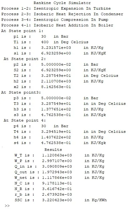
Case2 :-
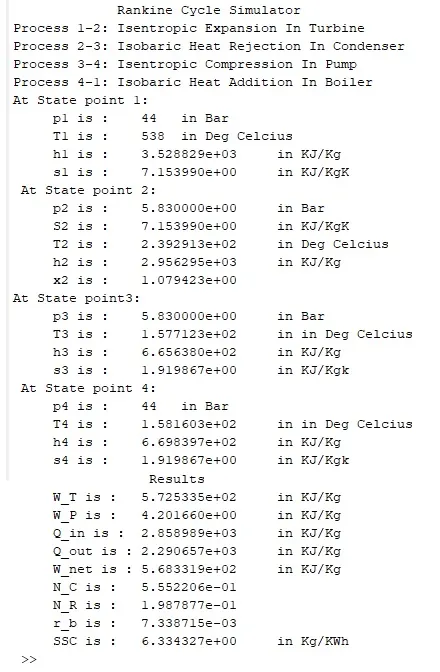
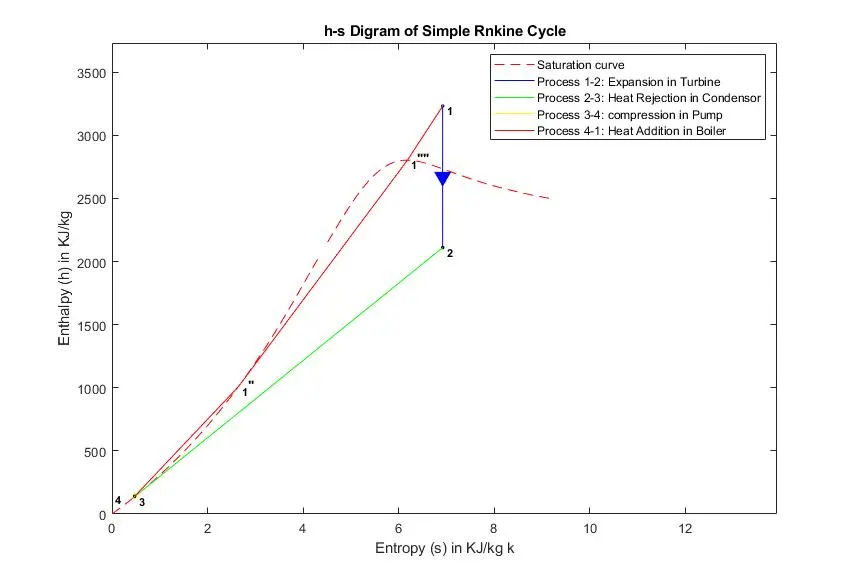
Plot Result:-
Case 1
Case 2
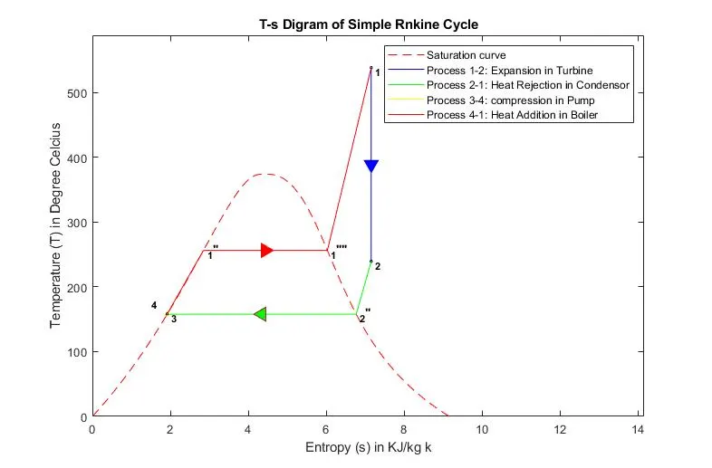
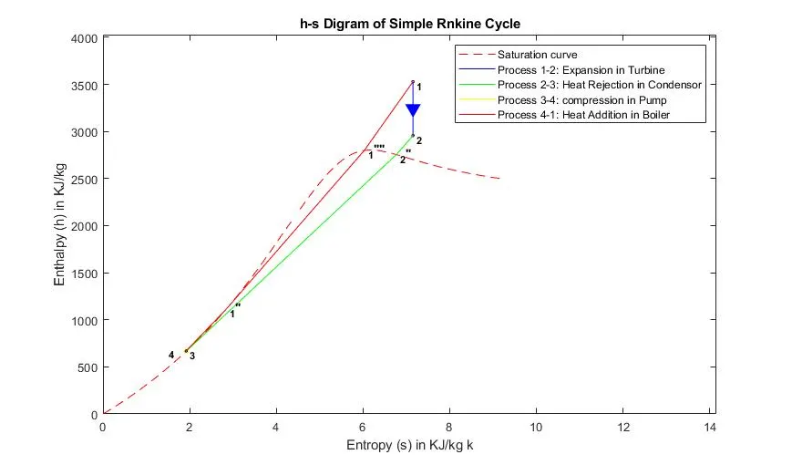
Errors in programs.
1. Here when calculating temperature at point 2 , we consider s2 = s1 which as per our theory process 1-2 is insntopic but in programing first i calcualte dryness fraction using s2, sf2 and sg2 if it is less then or equalt to one i.e. point 2 is inside the wet region(case1) else superheated region but the term drayness fraction is only for wet region and using this i calcualte h1(case1) but in superheated region to calcualte h1 either using theoritical formula or first using XSteam.m data. if i use the theoritical formula i get a small error with respect to XSteam.m data.
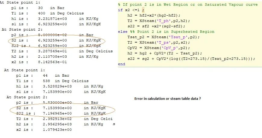
2. Now at point 3 and 4 agian same but this time we can't ignore it
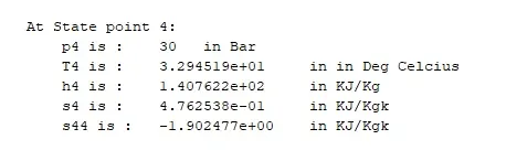
Here s44 is not be a right value of s4 because is may compresion is not isetropic (a real case senario) but it is impossible to -ve enropy value end of the process 3-4 as i already clear in thory.
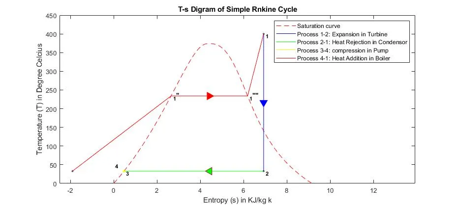
This error is may be due to units in formual is temperature in k but is XSteam.m date it is degree celcius or some other factor because every time it is different.
Result Conclusion:-
1. If we comapre both study study 1 give more net work output(allmost duble) in comparison of study 2. But per our theory if turbine inlet temperature is high turbine work, net work output is high and efficieny is also high. If you closely absorbe back work ratio in case2 is 3 times of back work ration of study 1 so pump work is also more as comare to study 2.
2. If we say why turbine work is not more in case 2 because temeprature is more so avalabele energy more so why turbine work less in study 2. This is because in study 2 at point 2 pressure is high as compare to study 1 and here at this point2 temperature is also high in study 2 so maximum posible work is less because temperature difference is less.
3. Here in case 1 carnot efficeny is 91.7% and rankine cycle efficeny is only 36%. Where in case 2 carnot efficeny is 55.5% and rankine cycle efficeny is 19.8%.
So can we say case1 is more efficient ?
NO
because in case 1 at that pressure and temperature conditions we can get effiency maximum upto 91.7% and we have of it's 1/3rd value but in case 2 at that pressure and temperature condition we ony get eficieny 55.5 % and get almost 20% or higher then it 1/3rd value.
So case 2 is better then one.
4. In case 1 condesor pressure is less then atmospheric pressure which is diffcult to maintain.
5. Specific steam consuption is more in case 2 so size of condesor is less.
6. Dryness fraction is more in casd2 or steam in turbine is complety dry or superheat so probabilty errosion or corosion of turbine blase is less as compare to case 1.
7. In case study 2 boiler pressure and temerature high , turbine temperature is high we need to use more strength and creap resistance material of construction which increase cost of installation but running cost is not so high because pump work is slightly high and heat suppy is slighty less but SSC is high and conesor size is lees which reduce the both the costs.
On the base of above points we conclude that case study 2 cycle plant is more sutaible to construct and operate.