Week 4 - CHT Analysis on Exhaust port

Aim:- Aim of this study to analysis the Conjugate Heat Transfer on a Exhaust Manifold of 4 cylinder Engine.

Introduction:- Conjugate heat transfer is a most common heat transfer phenomenon in which heat is transfer between solid and fluid both. It includes both conduction and convection heat transfer. Common application of this type of simulation includes cooling of electronics component and transformers, Heat exachange, cooling tower and bolider of a power plant, condensor of air conditioning system ect. In order to understand more about CHT so we choose a common practical application in Automobile industry that is Exhaust Manifold of 4 cylinder engine.

Now in this study we have a CAD model of Exhaust manifold with inlet hose having inlet boundary condition (v=5 m/s and T=700k).Here heat is transfer from hot fluid to ambient air at temperature equals to 300k and we assume the heat trnsfer coefficient at outer wall of manifold is 20 w/m2k and we have to calculate heat transfer coefficient at inner wall of manifold in ansys fluient and visualise the temperature and velocity contours.

Theory:-There are basically there modes of heat transfer

1. Conduction mode of HT :- Heat transfer between two point within a single type of body either solid or fluid. mosty we see conduction in solid bodies.for example heat transfer in a rod, slab ect
2. Convective mode of HT :- Heat transfer between different bodies or HT from one medium to another medium. Example radiators and finns in vehicles,heat exchanger etc.
3. Radition mode of HT :- It doesnot required any medium for its propogation and occures by electromeganetic wave propogation with speed of light. example soler radition in soler plants.

# Conjugate Heat transfer is a combination of both conduction and convection mode of heat transfer.Here first convection occure from internal fliud to the soild inner wall then conduction occure bitween inner wall and outer wall of manifold and then again heat is convected from outer wall to amient air.

Analysis procedure

1) PreProcessing

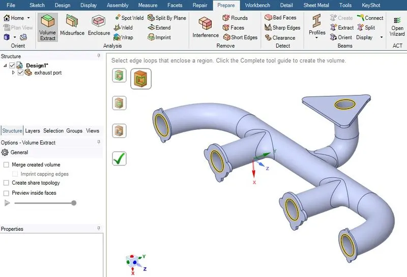
First import the model in Spacecalim and go go to prepaire tab click Extract volume the and active edge selection and select the cicumference of the inlet and outle ports and click the right button to extract the fluid voulme.

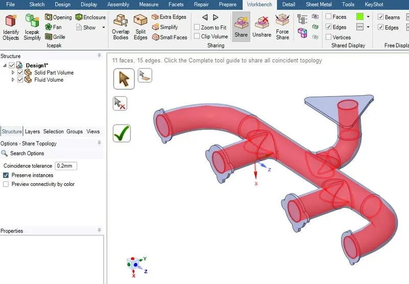
Now go to the Workbench Tab and click share to active share topology for mesh data tranfer between fliud and solid bodies.

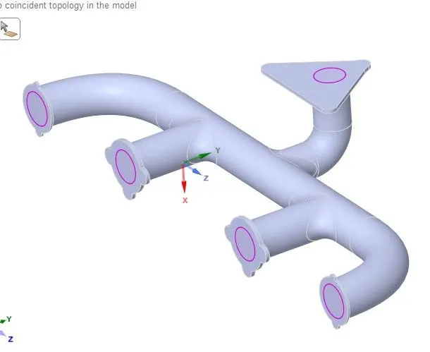
Now here we close the spaceclaim and open mesh environment and now before the generates the mesh we naming the boundaries.

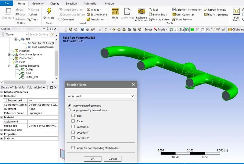
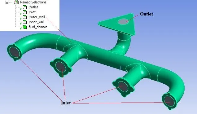
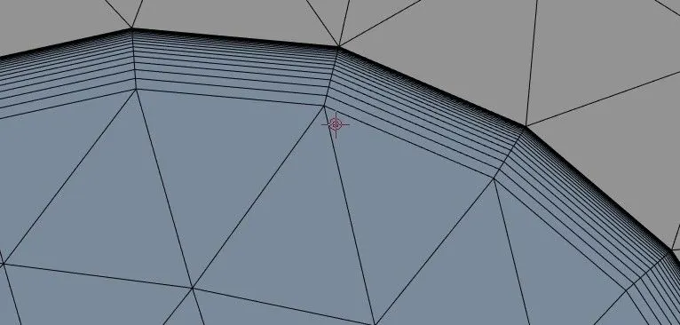
 Now here to capture boundary layer phenomina we have to provide inflation layer in meshing so we calculate first layer height and number of layes for groth factor 1.2

Now here flow is turbulent because this is an internal flow with Reynolds number grater then 2400

Re=rho*V*D/mu=51345

here i choose k-omega model because we have to capture flow parameter near to wall and for these condition k-omega model is best sutable model for this Y+ value thakes 1

now in Y+ calculator first layer height is

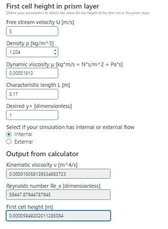
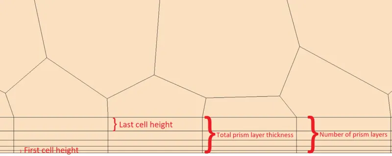
Now 

δ=△y(1-G^n)/(1-G)

so with this formula i got number of layers and get

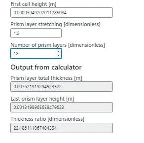
Now generate the mesh and check he quality also

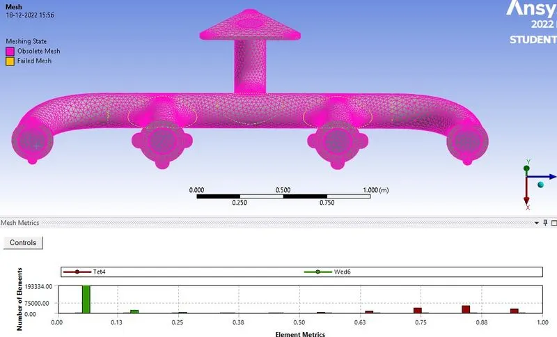
Here in quality check you can see element size of less then 0.13m having 193334 elemnts out 341234 elements i.e. mesh size is uniformaly mantaine in whole geometry.

If we zoom we can see the inflation layer neer the boundary and we also see how mesh data propogating from fluid to soild by maintaing element size at interation.

Now close the mesher and open the analysis setup

2 Solver setup

1) Material selection:- Now open the setup now first go to the cell zones and you can see both solid body and fluid volume.

here i select air as working fluid and aluminium for manifold solid body with their defult properties in ansys fluent data base.

2) Boundary conditions:- Now click boundaris and select the boundaries which we assine name in mesher

For Inlet velocity is 5 m/s and T is 700k

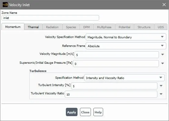
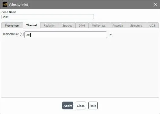
For outlet pressure is atmosperic pressure i.e. 0 gauge pressure and Temperature is 300K

And for outer pipe wall heat transfer coefficient is h=20 w/m2k and ambient temperature is 300k

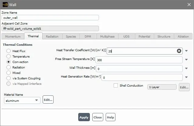
3) Model setup:- 

Select the Steady state analysis and pressure base solver 

check the Energy to calculate temperatur by solving energy equastion.

In Viscous select K-omega SST model without any changes click ok

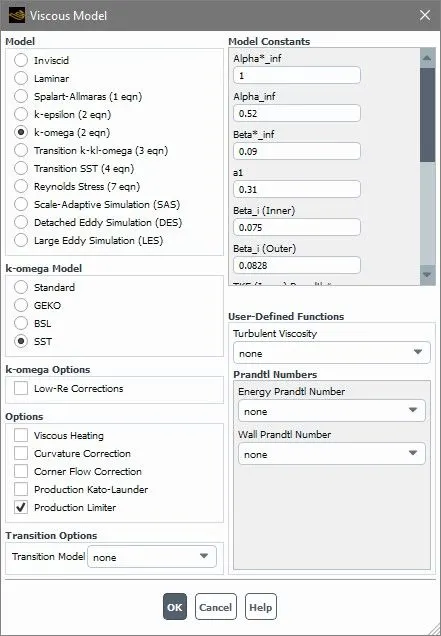
Here i chose K-omega model because i have to study flow parameters near to the wall.

4) Run analysis 

First initilize with hybrid meshod and then run analysis for 150 iterations.

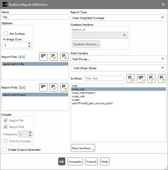
Before run analysis go to Defination>New>Surface Report>Area-Weighted Average

Type name as htc select inner wall shadow 

Note: Both inner wall and inner wall shadow are same surface but different in their direction so in result only change in the sign of value.

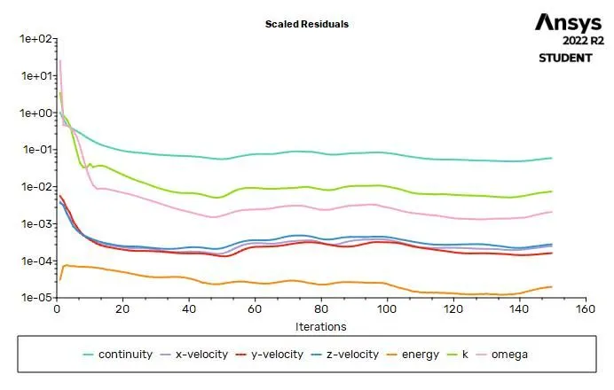
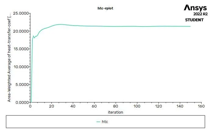
Here you can see in residula plot continuity equastion and k and omega are not converged but if you see htc-plot is become linear after 50 iteration so we can say our solution is converge.

Now i want to calculate htc minimum and maximum value by surface interigal and plot xy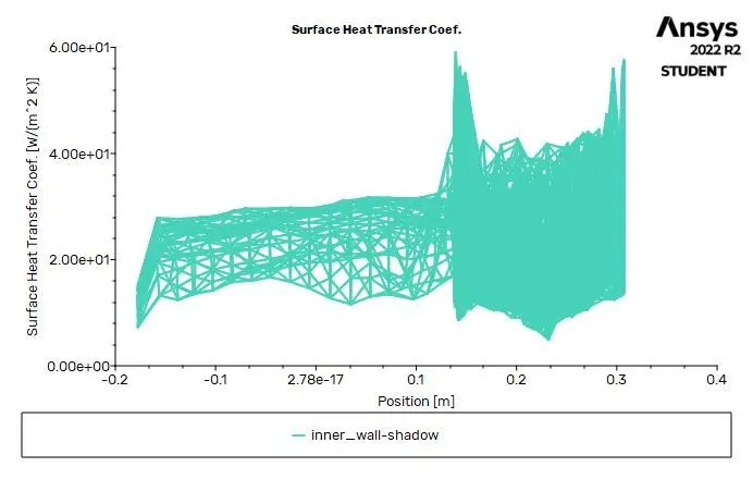 

##surface heat transfer coeffient at inner wall 

Maximum=123.32607 w/m2k

minmium=3.0521982 w/m2k

Average=21.313068 w/m2k

Now i check my result by analytical solution

1) BY corelation of dimentionless number Nu(Nusselt number)

Nu=conductive resistance by fluid/Surface conduction resistance

Nu=(D/KA)/1/(hA)=hD/K

Now here D is diamneter of pipe =150mm or 0.15m

K conductivity od fluid=0.0242w/mk

Now we can calculate Nu by corelaton 

Nu=0.023*Re^(0.8)*Pr^n

n is constant for cooing its value 3 and for heating it is 4

a) calculate Re=rho*v*D/mu

Re=(1.225kg/m3)*(5m/s)*(0.15m)/(1.789e-5kg/ms)=51345.25

b) calculating Pr=Kinematic diffusivity / thermal diffusivity= nue/alpha

nue=mu/rho=1.789e-5/1.225=1.46e-5

alpha=K/rho*cp =(0.0242 w/mk)/(1.225kg/m3)*(1006.43J/kgk)=1.96e-5m2/s

Pr=1.46e-5/1.96e-5=0.7454

c) Nu=0.023*51345.25^0.8*0.7454^0.3

Nu=0.023*5866.78*0.9156=123.54

d) h=Nu*K/D=123.54*0.0242/0.15=19.93W/m2k

and my numerical result is 21.313068W/m2k

error ((21.313-19.932)/19.932)*100=6.92% of error

2) By electrical analogy of heat transfer and cyclindrical cordiante system but this is very length method to solve

3 Post procedure

Now go to File mane> Export>Solution Data

Select the surfaces and select surface Heat Transfer coeffient, Temeprature static , Velocity amgnitude as quantites to export

Contour plot

1) velocity contours:- Here we plot conture on inlets and see only the fluid domain which you can see in below image Velocitis are not constant in joing pipe becouse of flow seperation.

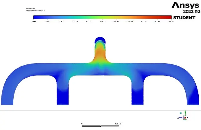
Velcoty contour at outlet you can see flow seperation at bend section and also see turbulance

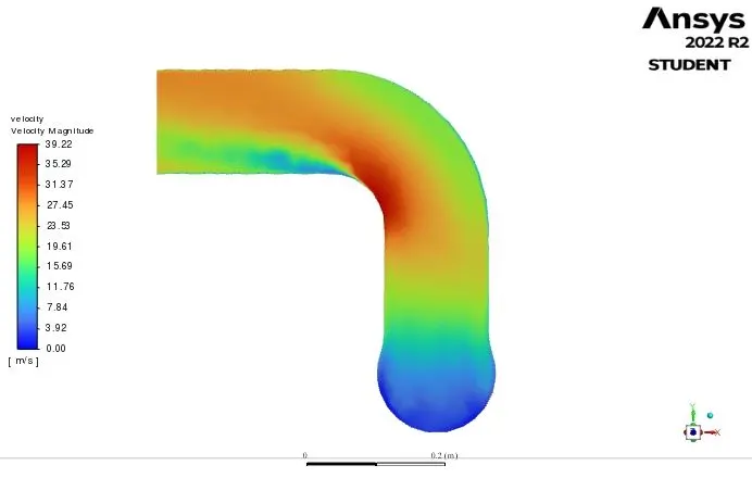
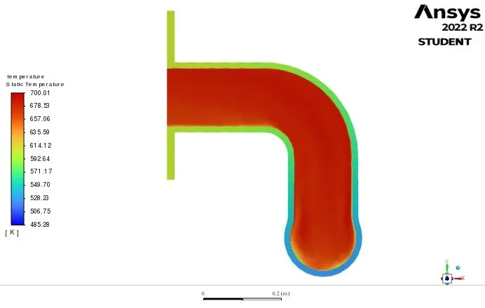
2 Temperature contour Here you can see Temperature dradient in both solid and fluid domain and you can see at bend temperature is less as compare to other so less heat conduct thought bend section, this becouse low velocity tends to low heat conduction at bend section.

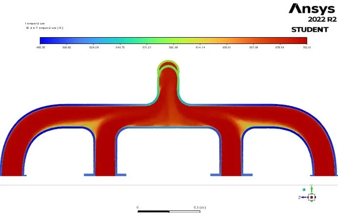
Tmperature contour at outlet here you can see easlity how conjugate heat transfer occure in joing section, where you see temperature contours is developing proprly and shoen bot convection in fliud domain and conduction in solid body.

Conclusion:-

Here Result comes with an error of around 7% which may be reduce by refining mesh or sizing mesh at inner wall, or by using different Y+ value instade of 1, we can choose it up to 5, but here here if we refine mesh ansys solver take more time to converged result and due fine meshing a lot of memory is consume by system so here we have to maintain y+ value and mesh size as per our requrement of time and system for the project.

Here if we increse inlet velocity the resultant convective heat transfer coefficient come with less error but after 10 m/s velcity, change convective heat transfer coefficien is less so we can say that with increse in velcity heat transfer is more but afetr few rage is heat transfer rate not change much more with increse in velocity.

Now choosing solver and model also effect my result accuracy, so if i choose k-epsilon model instade of k-omega result accuracy is less or error is more becuase here we have to calculate result near to surface.