Week 9 - Parametric study on Gate valve.

Aim:- To simulate flow through Gate valve in ansys fluent and perform a parametric study by setting the opening from 10% to 80%.

Theory:- A gate valve is the most common valve for water supply systems. It represents a linear-motion isolation valve and has a function to stop or allow the flow. Gate valves got their name from the closure element sliding into the flow stream to provide shutoff and, therefore, acting like a gate.

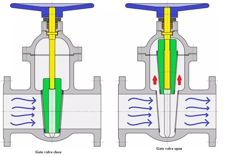
A gate valve is generally used to completely shut off fluid flow or, in the fully open position, provide full flow in a pipeline. Thus it is used either in the fully closed or fully open positions. A gate valve consists of a valve body, seat and disc, a spindle, gland, and a wheel for operating the valve.

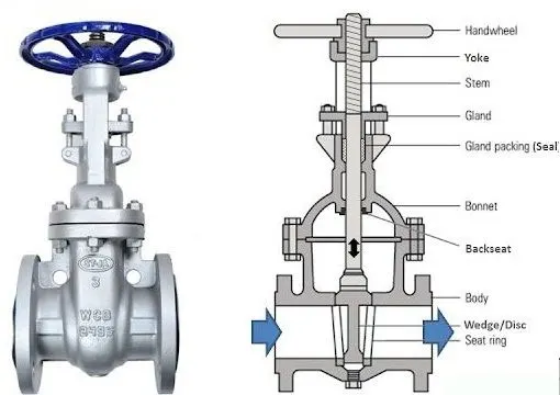
Typically featured in industries such as slurry, irrigation, mining, pharmaceuticals, power plants, oil, and gas, gate valves can connect and segregate media. Gate valves are thus named for the gate within the valve that slides on the valve seats to allow the flow of media. The gates are usually parallel and typically shaped into a knife or wedge. The stem of the valve indicates whether the valve is fully open or closed. Gate valves don’t leak in most cases although pressure-drop issues can prop. It’s a linear valve that’s popular for securely segregating the flow of media. It’s efficient where tight sealing is a must regardless of what the consistency of the media is. This type of valve isn’t used for regulating media as it might break down from the process. The lifespan of gate valve is extended by keeping them fully closed or open when in/out of use.

Procedure:-

(1) Pre processing:- In pre processing we first do modeling (i.e. creating fluid volume) and then go for meshing.

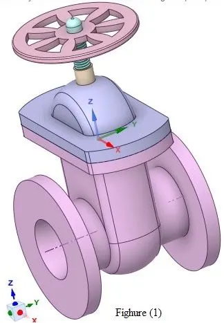
(a) Modeling:- In this step first open ansys space claimand imported the give model Step file by draging it to window.

Now this model contain some 3d solid, first we have component we have to create a fluid volume and then subtract the gate valve and spindle from it. But her for flow analysis we need pipe of 800mm length conected both side of the valve, so here we are not going to create pipe we just pull the vlave flange face as shown in figure (2).

For creating fluid volume go to Prepaire ribbon and click on extract fluid volume and active the edge selection and then select the edges as shon in figure (3).

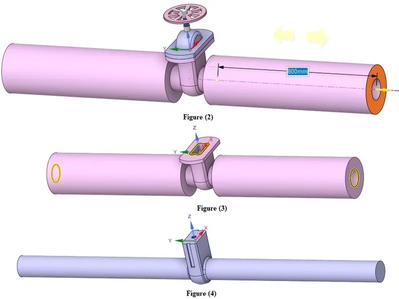
here we as shown in figure(4) is our require fluid volume, we can do first extract the volume then pull the fluid volume face but in that case if we go for parametric study as we update our geometry the 800mm face is gone so we have to againg do this so that i use this approach to pull the solid model face and then create fluid voume.

Paramerized the model:- Fot this first hide fluid volume and bottom componet from tree. Now in design ribbon click move, active componet selection click on gate disk an by pressing mid buttom opf mouse drag updarw and the value type 10mm as shown in below figure.

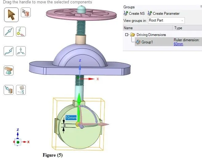
Now this 10mm we have to make parametrize, In ansys curren version we can don this by click on p button with dimention but here i go to Groups in tree as shown in above figure (5).

Now hide all componet and also suppres these solid bodies for physics but remember that we have to update our created fluid volume as per the our given parmeter for gate disk lift.

To performing right click fluid volume and click on Update volume body in context so that it update in the existing volume.

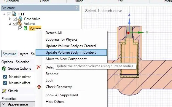
In above figure you can also see in section image how volume is updating as we lift the gate disk.

Now close the space claim.

(B) Meshing : Now open the meshing module generate the mesh

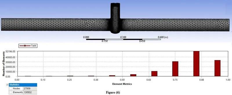
here number of elements are 130932, here we can do more presize mesing but here i use defult mesh parameter so that it takes optimum simulation time with the result.

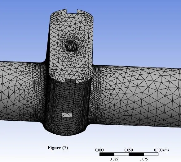
make sure that the generated mesh are fine at radiys and the hole by spindle.

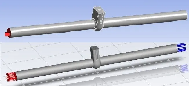
Now as shown in above figure we name the selection in meshing and ansys fluent with autometicaly assigned the boundary as shown in the above figure.

(2) Processing:-

Now here first go to Steup tree and first click General and fill these

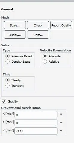
Solver Type: Pressure Based Solver

Gravity: -9.81 (in negative z-direction)

Solver: Steady State

here we use pressure base solver because our Mech number is less than 30. here you can fine velocity in solution clicking stander intilization then option and calculated velocity. But before this we have to create boundary condition

Boundary condtion:- Now we go to boundaries and select inlet and assine pressure inlet in type and gives value of inlet pressure 10pa as shown in below figure (8)

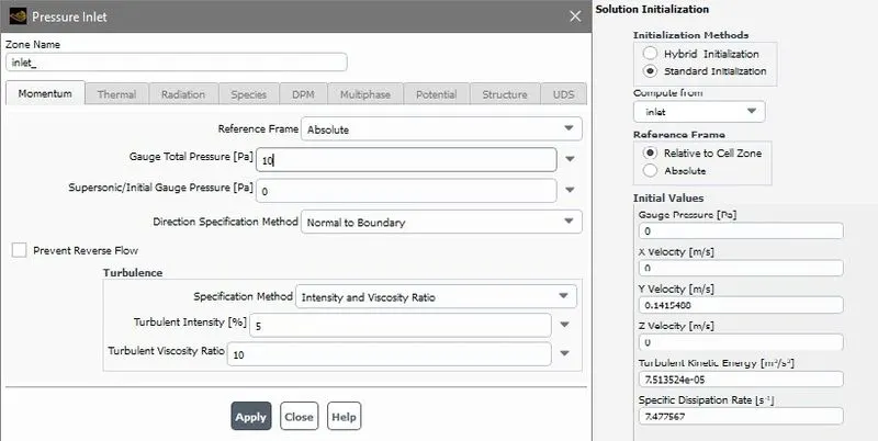
The oulet boundarie remain same pressure outlet at 1 atm pressure.

On basis of this inlet pressure we calculate velocity in y direction as shown in figure which is use to find mech number.

Physics :- Now in physics we select reaiazable k-epsillion model with scalable wall function as shown in figure (9).

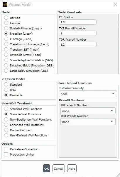
Now here we use reaiazable k-epsillion model because our studie is focused on near to the wall.

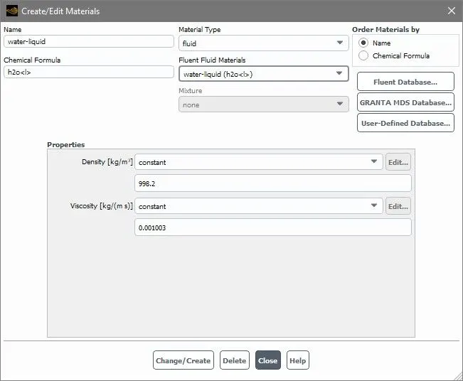
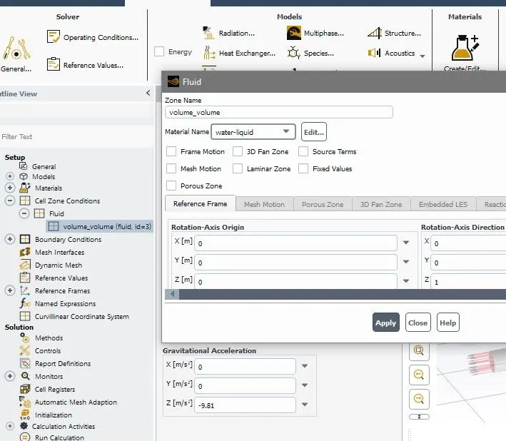
Material :- Now from fluent database select the water liquid material and in cell zone to fluid voulme define it as shown in below figures.

(3) Post Processing:-

Now create the out put parameter as Total pressure and mass flow rate at outlet.

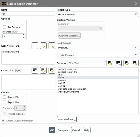
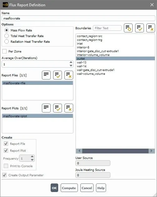
Now Creates a plane along the length so taht we can creates contoure plots for velocity and pressure.

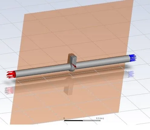
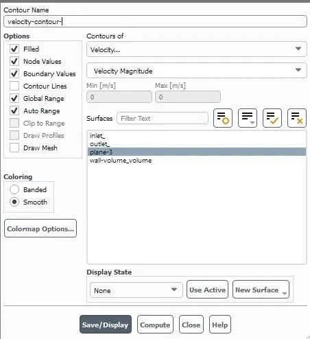
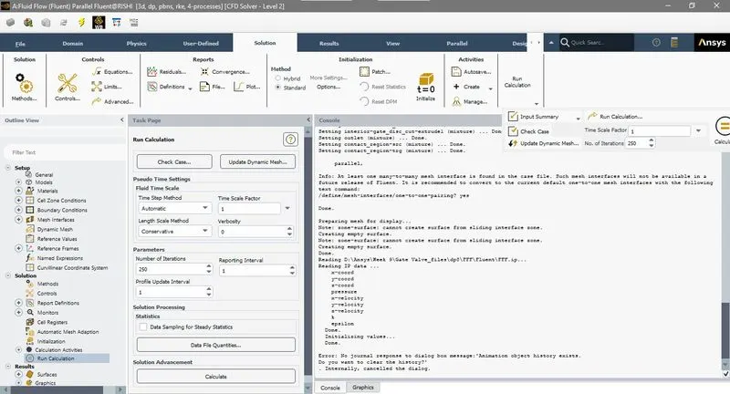
Now go to solution and Run anlysis at 250 iterations with standerd intilazation, we can also creates animation for velocity contours.

Parametric Study:- In previous part we crate on input parameter in space claim i.e. lift of gate disk and we also creates ouput parameter i.e. pressure and mass flow rate at outlet.

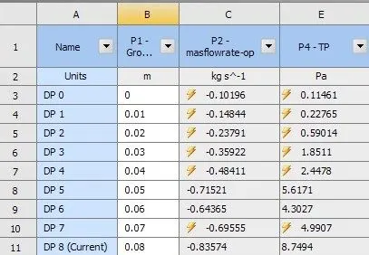
now for parametic study click on parameters now creating new data point in parametric study and after updating we get the output pressure and massflow rate at each data point

Results

(1)Residual plots:- In result first i show the residual plot for each case

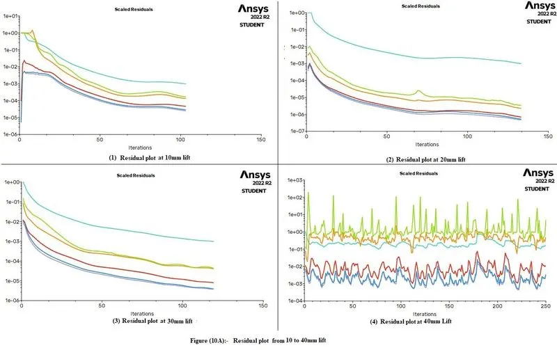
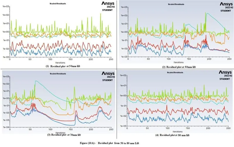
here you can see in case of lift from 10% to 30% our flow parameter simulation is stable and smoothley drop but after it it drops in zik zack way.

(2) Mass flow rate plot:- Here i required this so i plot it for each case

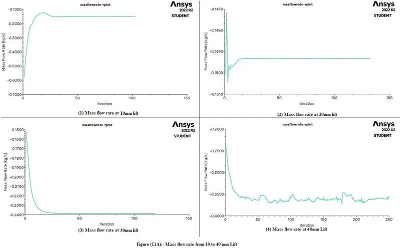
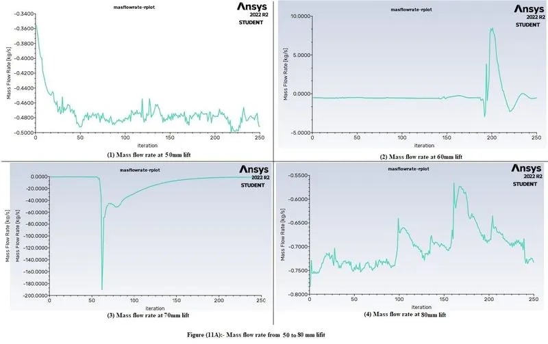
Countores:- Here i plot pressure and contoure for each case

Case1 10mm lift

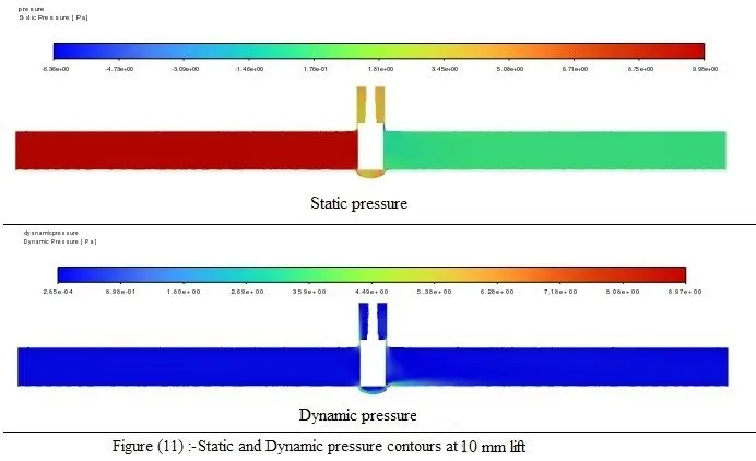
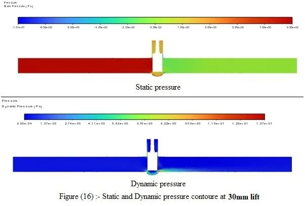
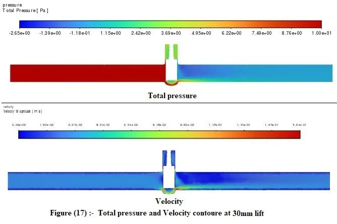
Here you can se ststic pressure at LHS is high then RHS because flow is from left to right but at vlave disk it restrict so ony there is pressure is varying and as you see dynamic pressure which is low and contant throuth the length only high at gate disk interface because here static pressure converted to dynamic pressure. If you see total pressure contoure which same as the static pressure. so pressure at outlet have more part of dyanmic as compare to static because static pressure at RHS is very low instade of dyanamic pressure.

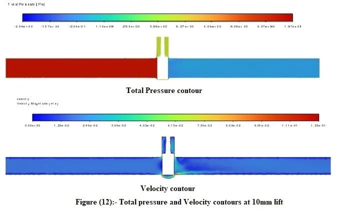
Here from this image we obsereved that total pressure is also decrease in RHS of gate disc.And from velocity contour you can see velocity is sligtly more after the disc.

Case2 - 20mm lift

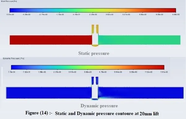
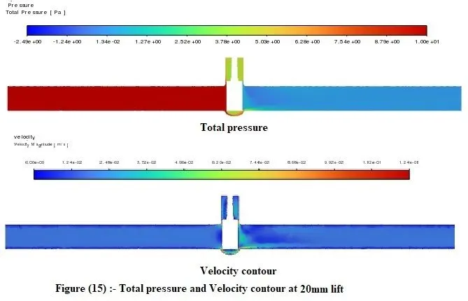
This same as privous results but ony some different at gate disk.

Case3 - 30mm lift

Case4 - 40mm lift

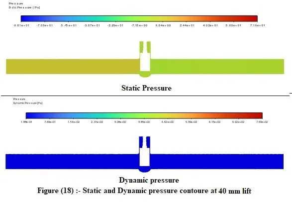
Now in this case Sligthly change in Left to Right hand side.

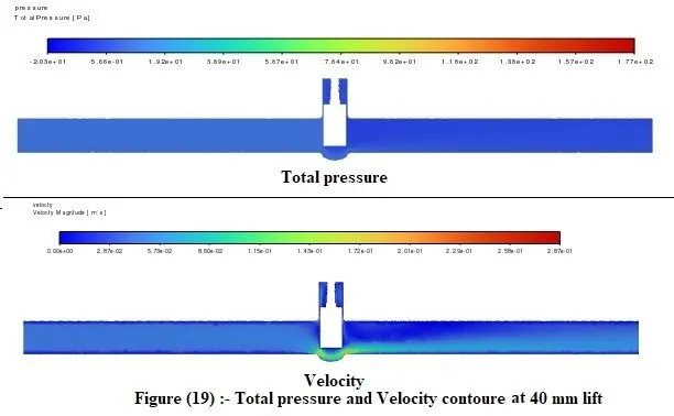
Case5 - 50mm lift

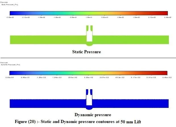
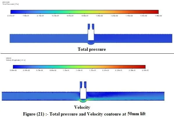
Case6 - 60mm lift

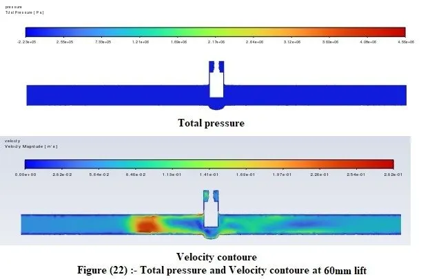
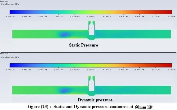
Here you can se some diffrent in flow which you never see in pressure contour but see in static and dynamic pressure contour. How static and dynbamic presure are converted to each other.

Case7 - 70mm lift

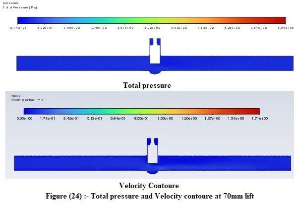
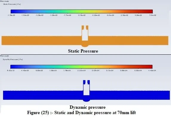
Now here Static and dynamic pressure both are constant throughut valve.

Case8 - 80mm lift

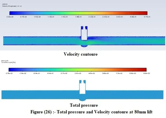
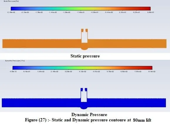
Part 2 :-Calculate the flow coefficient and flow factor for each opening and plot the graph.

Flow Coefficient:-The Flow Coefficient of a device is a relative measure of its efficiency at allowing fluid flow.

`C_v=Q*sqrt((S_g)/(triangleP))`

Q is Mass flow rate (expressed in US gallons per minute).

Sg is the specific gravity of water which is 1

△P is pressure drop (in PSI)

Flow factor:- The flow factor is the flow coefficient in metric units. It is defined as the flow rate in cubic meters per hour of water at a temperature of 16deg C with a pressure drop of 1 bar. It is given by the formula,

`K_v=Q*sqrt((S_g)/(triangleP))`

Where Kv - flow factor

Q - volume flow rate ( m3/hr )

SG - specific gravity of the fluid ( for water = 1 )

Δ⁢P">ΔP - pressure drop ( bar )

Now we can convert Kv to Cv by this formula

Cv=1.16*Kv

Now from ansys parametric study we get these data

Put these data and formula in table we get

lift in %	Pr. at inlet (pa)	Pr. at outlet (pa)	ΔP (pa)	ΔP (bar)	Mass flow rate (kg/s)	Mass flow rate (m3/hr)	Flow factor (Kv)	Flow coefficent (Cv)
0	10	0.11461	9.88539	0.0000988539	0.10196	0.3677178922	36.98433874	42.90183293
10	10	0.22765	9.77235	0.0000977235	0.14844	0.5353476257	54.15472745	62.81948384
20	10	0.59014	9.40986	0.0000940986	0.23791	0.8580204368	88.4516729	102.6039406
30	10	1.8511	8.1489	0.000081489	0.35922	1.295523943	143.5145553	166.4768841
40	10	2.4778	7.5222	0.000075222	0.48411	1.74593869	201.3059219	233.5148694
50	10	5.6028	4.3972	0.000043972	0.71521	2.579398918	388.9828049	451.2200537
60	10	4.3037	5.6963	0.000056963	0.64365	2.321318373	307.5659699	356.776525
70	10	4.9907	5.0093	0.000050093	0.69555	2.508495292	354.4253438	411.1333988
80	10	8.7494	1.2506	0.000012506	0.83574	3.014089361	852.3086809	988.6780699

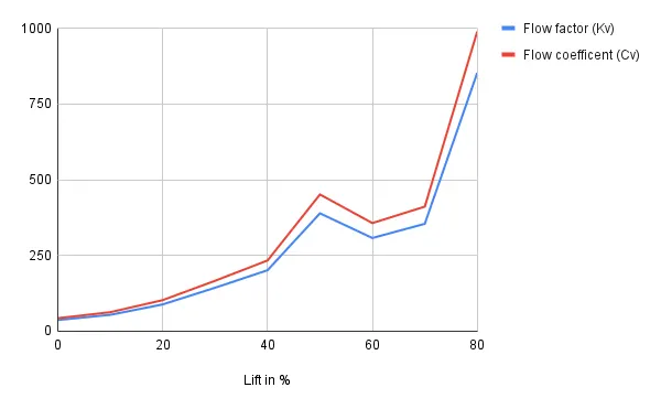
By useing above table we plot graph

Conclusion

1. From this challange we understand how static and dynamic pressure change when in a flowing pipe we add gate valve with different opening precentage. And pressure at outlet have more contribustion of dynamic pressure instade of ststic.

2. Pressure difference throughout the gate valve decreases with increasing opening percentage. This is because as we lift the valve disc which is obstacles in flow at that point genrated dynamic pressure is decreases and because of this total pressure at outlet is decresaes.

3. From above table we conclude that mass-flow rate and velocity increase with increasing opening percentage. This is because there are more pathways for the water to flow.

4. Flow factor and flow coefficent are linearly increase with opening percentage but from graph we can see some regration points this is because of some amount of turbulence due to sharp edge of valve disc so that we can say gate valve should operate in a fully-opened or fully-closed position. A partially-opened valve induces vibration which can damage the gate valve.

5. Also the gate valve should be closed gradually rather than suddenly, as it causes a water hammer effect which can again damage the gate valve.