Week 4.1 - Solving second order ODEs

Objective :- Obejective of this study is to

1) Solve 2nd order diffrential equastion for simple pendulum and plot graph for angular displacement and angular velocity at each time value.

2) Animate the oscillation of simpe pedulumn.

Theory :-A pendulum in simple harmonic motion is called as 'Simple Pendulum". It is consisting of a mass 'm' hanging from a light weight (negligible weight) string of length 'l' and fixed at a pivot point and damping coefficient 'b'. When it is displaced from its resting or equilibrium position it is subjected to a restoring force due to gravity that will accelerate it back toward europium position, when released, restoring forces acting on pendulum mass cause it to oscillate about muralism position.

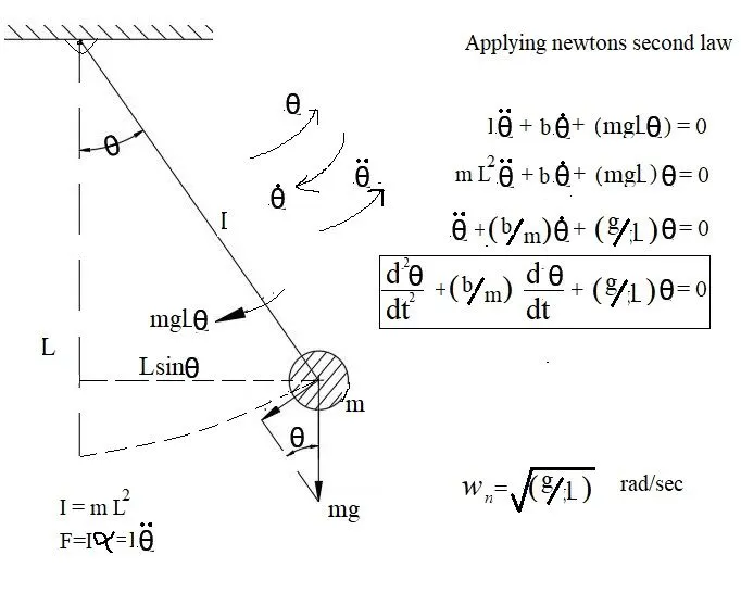
In the above equation,

g = gravity in m/s2,

L = length of the pendulum in m,

m = mass of the ball in kg,

b=damping coefficient.

we have to given in question

L=1 metre,

m=1 kg,

b=0.05.

g=9.81 m/s2.

and we have to Simulate the motion between 0-20 sec, for angular displacement=0,angular velocity=3 rad/s at time t=0

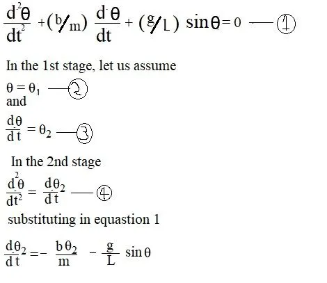
Matlab code for solving 2nd order differential equastion

% Solving 2nd order diffrential equation for simple pedulum
clear all
close all
clc

% Input data
L=1;
m=1;
g=9.81;
b=0.5;
% Initial condition 
% At time t=0 , angular velocity =3 rad/sec

theta_0=[0;3];

% Time space defination

T=linspace(0,20,100);

%silving ODE
[t,result]=ode45(@(t,theta) ode_fun_sp(t,theta,b,g,L,m),T,theta_0);


%plot
figure(1)
plot(t,result(:,1))
hold on 
plot(t,result(:,2))
xlabel('Time')
ylabel('Plot')
grid on
legend('Angular displacement','Angular velocity')

1) Input data:- here in above code first we give input data for program.For this we assine values of varible b,g,L&m.

code

b=0.5;

g=9.81;

L=1;

m=1;

2) Initial condition:- in the second part of program we give initial condition.

here intial condition is

At time t=0 sec

angular displacement = 0

angular velocity=3 rad/sec

for assining this we make a matrix of 2x1

code

theta_0=[0;3];

3) Defining time space:- Here we define a time space of span T.

this time space have 100 value in between 0 to 20 sec time span.

code

T=linspace(0,20,100);

4) Defining Function in another script:- Now we define function for our ode in another script.or we can say we define an external function for our ODE.

code

function[theta_dot]=ode_fun_sp(t,theta,b,g,L,m)
theta1=theta(1); % from equastion no 2
theta2=theta(2);
theta1_dot=theta2; % from equastion no 3
theta2_dot=-(b/m)*theta2-(g/L)*sin(theta1);
theta_dot=[theta1_dot;theta2_dot]
end

in the first line we call a function name "ode_fun_sp" whith varible t,theta,b,g,L,m.

here we assine the value of elements of 'theta' matrix to theta1 & theta2.

and then

theta1_dot = theta2 % from equastion 3

and assine theta _double_dot=theta2_dot % from equastion 4

and write the 2nd order diffrential equastion

Here in output of this function we get a matrix [theta_dot] which has 2 values of 'theta_dot'

5) Solving ODE using ode45:-Now we came back to our main program and write syntex of solving ode

[t,result]=ode45(@(t,theta) ode_fun_sp(t,theta,b,g,L,m),T,theta_0);

here from this code we get 2 values of theta_dot for each time step in command window. from these 1st value shows Angular displacement and second Shows Angular velocity.

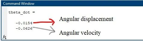
these value are store in matric [t,result]

here for each value of t there are two value of result.

these matrix [t,result] is 100x3 matrix which have 100 values of t ,result1 and result2.

6) Ploting graph:-in the last section of code we try to plot graph here in first code we plot a graph between time t and and first values of result.and then second plot is a graph of time t and second values of result.

code

%plot
figure(1)
plot(t,result(:,1))
hold on 
plot(t,result(:,2))
xlabel('Time')
ylabel('Plot')
grid on
legend('Angular displacement','Angular velocity')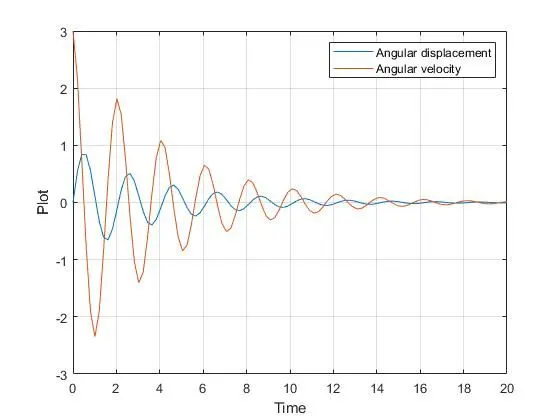

7) Animate the oscillation of simpe pedulumn :-

code

% Animate the oscillation of simpe pedulumn

ct=1;
for i=1:length(result)
    Angle=result(i,1);
    x_0=0;
    y_0=0;
    x_1=1*sin(Angle);
    y_1=-1*cos(Angle);
    figure(2)
    plot(x_1,y_1,'.','markersize',100,'color','g');
    hold on
    plot([x_0,x_1],[y_0,y_1],'color','b','linewidth',2);
    plot([-1,1],[0,0],'color','r');
    axis([-1 1 -1.2 0.2])
    hold off
    M(ct)= getframe(gcf);
    ct=ct+1;
end
movie(M)
videofile = VideoWriter('simplependulum.avi','uncompressed AVI');
open(videofile)
writeVideo(videofile,M)
close(videofile)

In the above code first we define a counter ct

and make a for loop such that when we execute this we get coordinates of x_1,Y_1.

then we plot this for each time frame.and now we capture the frame using (gcf) get frame command.

now we assine a array M for movie

and write video file and save it name 'simplepedulumn.avi'

after run this program file will save in our current folder.

Error in code writing:-

while ploting if you dont give pauese or hold on and hold off you plots are not is a squeence of animation.

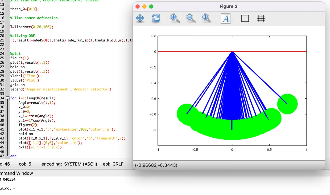
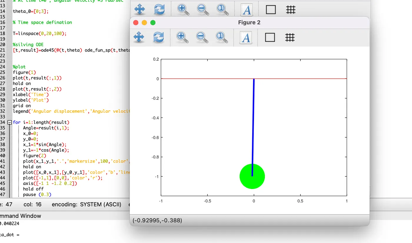
Conclusion :- Here colclusion from our grap and video

1).The plot of angluer displacement is a sine a wave where as plot of angluer velocity is cosine a wave.i.e. When anguler displacement is zero (equllibrim position) angular velocity is maximum and when anguler displacement is maximun (end position) angular velocity is zero.This will we observed in our simlation.

2).The plot also observed anguler displacement and angluer velocity have exponentially decreasing graph with time it shows that the amplitute of the waves is reducing. It is because of friction or damping.Now in animation the swing of pendulum is also reduce by time