Week 9 - FVM Literature Review

Finite Volume Method(FVM):- This is a discreatization method use for linearization of PDE of fluid flow (i.e. Navior-stokes equestion). In this tequinic unit volume called as grid is to be considered for solving governing equestion and varible properotes at notes are pressure, velocity and temperature ect.

FVM uses a volume integral formulation of the problem with a finite partitioning set of volumes to discretize the equations. FVM is in common use for discretizing computational fluid dynamics equations.

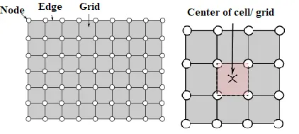
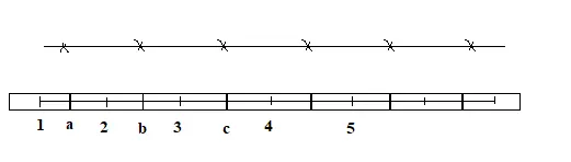
In FDM we cosider node ponits here we consider center points

In this mehod first we do volume intergal of govrning equastion. for example if we have linear heat conduction equastion

`del/(delx)(alpha(delT)/(delx))+S=0`

`oint( del/(delx)(alpha(delT)/(delx))+S)dV=0`.........(1)

`[ alpha(delT)/(delx)]_b ^a +SdV=0`

`alpha_bA[(T_3-T_2)/(trianglex)]-alpha_aA[(T_2-T_1)/(trianglex)]+Sdx=0`.........(2`

Finite difference Method(FDM):-A finite difference method (FDM) discretization is based upon the differential form of the PDE to be solved. Each derivative is replaced with an approximate difference formula that can generally be derived from a Taylor series expansion or taylor Table method.

# Difference between FVM and FDM

1. The FDM is easiest to understand when mesh is structured and in Cartesian coordinates system. For unstructured mesh FVM is easier as copaire to FDM because in FDM we have to define a maping function for a different varible space of ν and ε similar to cartesian space of x and y and solve equation for this space then use transformation function for converting result form ν and ε to x and y.
2. In Finite Differnece, the Dependant variable values are stored at the nodes only.But in FVM, the dependant values are stored in the center of the cell.
3. In FDM we deals with differential foam of governing equarion where as in FVM we deals with intergral foam of governing equastion.
4. With FDM we can solve both type of equastion either conservative or nonconservative but in FVM we only deals with conservative foam of governing equastion.
5. For 3D and moving grids FVM is much better then FDM.

# Need of interpolation in FVM

As we can observed in equastion (1), it contains both surface and volume intergals and in FVM we have to solve this intergral at center points of cell instade of nodes points as shown in figure.

Now we have ony value of T_0 and T_N , which is our bounday conditions so in FVM we apply a scheme to entire region in shuch a way we calculate temeerature at intermindates nodes alos.we can use either FDS or BDS and CDS for discreatizing the volume.

`alpha_bA[(T_2-T_1)/(trianglex)]-alpha_aA[(T_1-T_0)/(trianglex)]+Sdx=0`.........(3)` FD`

if

S is linear varitation S=a+bT

`alpha_bA[(T_2-T_1)/(trianglex)]-alpha_aA[(T_1-T_0)/(trianglex)]+(a+b.T_1)trianglex=0`.........(4)`

# Flux limiters

Flux limiters are used in high resolution schemes, a numerical schemes used to solve problems in science and engineering, particularly fluid dynimics, described by PDEs.

The flux limiters are also referred to as slope limiters because they both have the same mathematical form, and both have the effect of limiting the solution gradient near shocks or discontinuities.

The main idea behind the construction of flux limiter schemes is to limit the spatial derivatives to realistic values – for scientific and engineering problems this usually means physically realisable and meaningful values

They are used in high resolution schemes, for solving problems described by PDEs and only come into operation when sharp wave fronts are present. For smoothly changing waves, the flux limiters do not operate and the spatial derivatives can be represented by higher order approximations without introducing spurious oscillations.

`alpha_bA[(T_2-T_1)/(trianglex)]-alpha_aA[(T_1-T_0)/(trianglex)]+(a+b.T_1)trianglex=0`.........(4)`

in this equastion we use `T_(i+1/2)=T_(i+1/2)^(low)-phi(x)(T_(i+1/2)^(low)-T_(i+1/2)^(high))` and`T_(i-1/2)=T_(i-1/2)^(low)-phi(x)(T_(i-1/2)^(low)-T_(i-1/2)^(high))` instade of T_1 and T_0 when our finding at node 1/2.

here `T_(i+1/2)^(low)`and `T_(i+1/2)^(high)` are low and high resolution flux of Tempereture. and `phi(x)` is flux limiting function.