Week 3.5 - Deriving 4th order approximation of a 2nd order derivative using Taylor Table method

Aim:- Aim of this study is to derive the fourth order approximation of a second order derivative using central and skewwd differencing schemes with help of taylor table method and compare it with the analytical derivative for the given function.

Objective:-
1) To derived fourth order approximations of a second order derivative using central differencing,skewed right sided differencing and skewed left sided differencing and also prove that skewed schemes are fourth order or not.

2) Write a matlab script to evaluate the second order derivative of the analytical function exp(x)*cos(x) and compare with the central differencing,skewed right sided differencing and skewed left sided differencing numerical scheme.and also plot absolute error between these schemes.

3) And explain difference between central and skewed schemes.

Theory :- In this study first we have to derive expression for the numerical schemes of 4th order approximation of second order derivative.

A) Central Differencing scheme:-

Here

The order of accuracy P = Number of nodes in the stencil N - order of derivative Q + 1

then

Number of nodes in the stencil N=The order of accuracy P + order of derivative Q - 1

Now we required 4th order accuracy for 2nd order derivative

then

Number of nodes in the stencil N= 4+2-1=5

since we know Number of nodes in the stencil is 5, then our numerical stencial look in this scheme

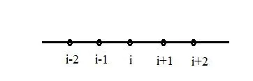
Here, we are computing 4th oder approximation at point (i), where we take information from the four point surrounging (i), i.e. we take two point from left side {(i-2) & (i-1)}and two from right side {(i+1) & (i+2)} of (i).and the distance between each point is Δx.

base on this stencil our hypothesis function is

for calculating values of coefficents a,b,c,d,e. first we write taylor series for each term in our equastion (1).

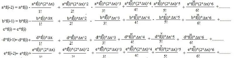
Now assemble this we put above terms in our hypothesis equastion (1)

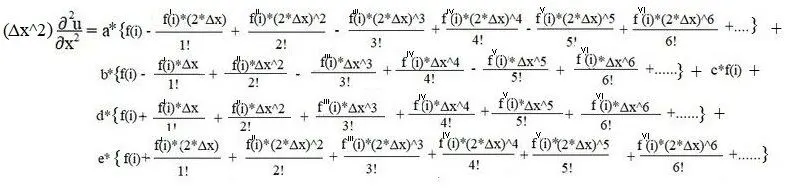
Arrange in Taylor table foam

stesial\terms	f(i)	Δx f'(i)	Δx^2 f''(i)	Δx^3 f"'(i)	Δx^4 f"''(i)	Δx^5 f'""(i)	Δx^6 f'""'(i)
a*f(i-2)	a	-2a	4a/2	-8a/6	16a/24	-32a/120	64a/720
b*f(i-1)	b	-b	b/2	-b/6	b/24	-b/120	b/720
c*f(i)	c	0	0	0	0	0	0
d*f(i+1)	d	d	d/2	d/6	d/24	d/120	d/720
e*f(i+2)	e	2e	4e/2	8e/6	16e/24	32e/120	64e/720
Sum	0	0	1	0	0	?	?

Here we have five equastion so we get ony 5 unknows a,b,c,d,e and in table we assume only first five term in our hypothesis and we cant't say about other term's .

Now we want to calculating f''(i) to we take summation of f''(i) is equal to 1 and summation of f(i),f'(i),f"'(i) and f""(i) is zero.

Therefore

a+b+c+d+e=0 ......(i)

-2a-b++d+2e=0 ....(ii)

2a+(b/2)+(d/2)+2e=1 ...(iii)

(-8a/6)-(b/6)+(d/6)+(8e/6)=0 ....(iv)

(16a/24)+(b/24)+(d/24)+(16e/24)=0 .....(v)

Now write above system of linear equastions in matrix foam [A][x]=[B]

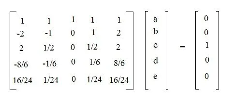
Now solving matrix in matlab

% [A][x]=[B]

% [x]=inv[A]*[B]

A=[1,1,1,1,1;-2,-1,0,1,2;2,1/2,0,1/2,2;-8/6,-1/6,0,1/6,8/6;16/24,1/24,0,1/24,16/24]

A =

1.0000 1.0000 1.0000 1.0000 1.0000
-2.0000 -1.0000 0 1.0000 2.0000
2.0000 0.5000 0 0.5000 2.0000
-1.3333 -0.1667 0 0.1667 1.3333
0.6667 0.0417 0 0.0417 0.6667

B=[0;0;1;0;0]

B =

0
0
1
0
0

C=inv(A)*B

C =

-0.0833
1.3333
-2.5000
1.3333
-0.0833

rats(C) % For getting coefficent values in rational numbers

ans =

5×14 char array

' -1/12 '
' 4/3 '
' -5/2 '
' 4/3 '
' -1/12 '

then

a = -1/12
b =4/3
c = -5/2
d =4/3
e = -1/12

Here we notice that a=e and d=b

Now again from our hypothesis eq.(1) with taylor series expansion of f(i-2),f(i-1),f(i),f(i+1)&f(i+2)

To get second order derivative put the coefficent of f''(i) is equal to 1 and coefficents of f(i),f'(i),f"'(i),f""(i) and f""'(i) is equal to zero.

then

Here coefficent of f""'(i) is become zero because a=e and b=d

Dividing by Δx^2

Now we know that the order of truncation error term is define as the order of approximation so we can say that the above expression is the 4th order approximation of 2nd order derivative.

After putting value of a,b,d,&e our final expression is

B) Skewed Right side Differencing scheme:-

Here

The order of accuracy P = Number of nodes in the stencil N - order of derivative Q

then

Number of nodes in the stencil N=The order of accuracy P + order of derivative Q

Now we required 4th order accuracy for 2nd order derivative

then

Number of nodes in the stencil N= 4+2=6

since we know Number of nodes in the stencil is 6, then our numerical stencial look in this scheme

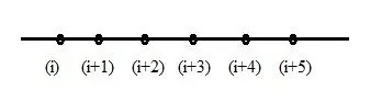
Here, we are computing 4th oder approximation at point (i), where we take information from the five point next to (i) and the distance between each point is Δx.

base on this stencil our hypothesis function is

Taylor series expansion of each term

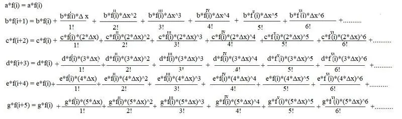
Now assemble this we put above terms in our hypothesis equastion (2) and arrange in taylor table

stesial\terms	f(i)	Δx f'(i)	Δx^2 f''(i)	Δx^3 f"'(i)	Δx^4 f"''(i)	Δx^5 f'""(i)	Δx^6 f'""'(i)
a*f(i)	a	0	0	0	0	0	0
b*f(i+1)	b	b	b/2	b/6	b/24	b/120	b/720
c*f(i+2)	c	2c	4c/2	8c/6	16c/24	32c/120	64c/720
d*f(i+3)	d	3d	9d/2	27d/6	81d/24	243d/120	729d/720
e*f(i+4)	e	4e	16e/2	64e/6	256e/24	1024e/120	4096e/720
g*f(i+5)	g	5g	25g/2	125g/6	625g/24	3125g/120	15625g/720
Sum	0	0	1	0	0	0	?

Here we have six equastion so we get ony 6 unknows a,b,c,d,e,g and in table we assume only first five term in our hypothesis and we cant't say about other term's .

Now we want to calculating f''(i) to we take summation of f''(i) is equal to 1 and summation of f(i),f'(i),f"'(i),f""(i) and f""'(i) is zero.

Therefore

a+b+c+d+e+g=0 ......(i)

0+b+2c+3d+4e+5g=0 ....(ii)

0+(b/2)+(4c/2)+(9d/2)+(16e/2)+(25g/2)=1 ....(iii)

0+(b/6)+(8c/6)+(27c/6)+(64e/6)+(125g/6)=0 ....(iv)

0+(b/24)+(16c/24)+(81d/24)+(256e/24)+(625g/24)=0 .....(v)

0+(b/120)+(32c/120)+(243d/120)+(1024e/120)+(3125g/120)=0 .....(vi)

Now write above system of linear equastions in matrix foam [A][x]=[B]

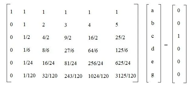
Solving in matlab

>> A=[1,1,1,1,1,1;0,1,2,3,4,5;0,1/2,4/2,9/2,16/2,25/2;0,1/6,8/6,27/6,64/6,125/6;0,1/24,16/24,81/24,256/24,625/24;0,1/120,32/120,243/120,1024/120,3125/120]

A =

1.0000 1.0000 1.0000 1.0000 1.0000 1.0000
0 1.0000 2.0000 3.0000 4.0000 5.0000
0 0.5000 2.0000 4.5000 8.0000 12.5000
0 0.1667 1.3333 4.5000 10.6667 20.8333
0 0.0417 0.6667 3.3750 10.6667 26.0417
0 0.0083 0.2667 2.0250 8.5333 26.0417

>> B=[0;0;1;0;0;0]

B =

0
0
1
0
0
0

>> inv(A)*B

ans =

3.7500
-12.8333
17.8333
-13.0000
5.0833
-0.8333

>> rats(ans) % For getting coefficent values in rational numbers

ans =

6×14 char array

' 15/4 '
' -77/6 '
' 107/6 '
' -13 '
' 61/12 '
' -5/6 '

therefore

a =15/4
b =-77/6
c =107/6
d =-13
e =61/12
g =-5/6

Now from our hypothesis eq (2) with taylor series expansion of f(i),f(i+1),f(i+2),f(i+3),f(i+4) & f(i+5).

To get second order derivative put the coefficent of f''(i) is equal to 1 and coefficents of f(i),f'(i),f"'(i),f""(i),f""'(i) and f"'"'(i) is equal to zero.

then dividing equastion by Δx^2

Now here again in above expression the truncation error term is of 4th order then this is also 4th order approximation of 2nd order derivative.

After putting value of a,b,d,e&g our final expression is

C) Skewed Left side Differencing scheme:-

Here

The order of accuracy P = Number of nodes in the stencil N - order of derivative Q

then

Number of nodes in the stencil N=The order of accuracy P + order of derivative Q

Now we required 4th order accuracy for 2nd order derivative

then

Number of nodes in the stencil N= 4+2=6

since we know Number of nodes in the stencil is 6, then our numerical stencial look in this scheme

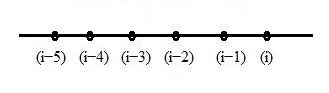
Here, we are computing 4th oder approximation at point (i), where we take information from the five point privious to (i) and the distance between each point is Δx.

base on this stencil our hypothesis function is

Taylor series expansion of each term

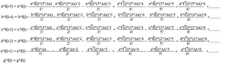
Now assemble this we put above terms in our hypothesis equastion (2) and arrange in taylor table

stesial\terms	f(i)	Δx f'(i)	Δx^2 f''(i)	Δx^3 f"'(i)	Δx^4 f"''(i)	Δx^5 f'""(i)	Δx^6 f'""'(i)
a*f(i-5)	a	-5a	25a/2	-125a/6	625a/24	-3125a/120	15625a/720
b*f(i-4)	b	-4b	16b/2	-64b/6	256b/24	-1024b/120	4096b/720
c*f(i-3)	c	-3c	9c/2	-27c/6	81c/24	-243c/120	729c/720
d*f(i-2)	d	-2d	4d/2	-8d/6	16d/24	-32d/120	64d/720
e*f(i-1)	e	-e	e/2	-e/6	e/24	-e/120	e/720
g*f(i)	g	0	0	0	0	0	0
Sum	0	0	1	0	0	0	?

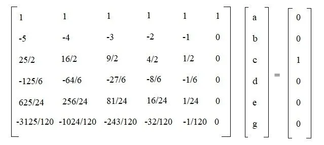
Solving in Matla

>> A=[1,1,1,1,1,1;-5,-4,-3,-2,-1,0;25/2,16/2,9/2,4/2,1/2,0;-125/6,-64/6,-27/6,-8/6,-1/6,0;625/24,256/24,81/24,16/24,1/24,0;-3125/120,-1024/120,-243/120,-32/120,-1/120,0]

A =

1.0000 1.0000 1.0000 1.0000 1.0000 1.0000
-5.0000 -4.0000 -3.0000 -2.0000 -1.0000 0
12.5000 8.0000 4.5000 2.0000 0.5000 0
-20.8333 -10.6667 -4.5000 -1.3333 -0.1667 0
26.0417 10.6667 3.3750 0.6667 0.0417 0
-26.0417 -8.5333 -2.0250 -0.2667 -0.0083 0

>>inv(A)*B

ans =

-0.8333
5.0833
-13.0000
17.8333
-12.8333
3.7500

rats(ans) % For getting coefficent values in rational numbers

ans =

6×14 char array

' -5/6 '
' 61/12 '
' -13 '
' 107/6 '
' -77/6 '
' 15/4 '

therefore

a =-5/6
b = 61/12
c = -13
d =107/6
e =-77/6
g =15/4

Now from our hypothesis eq (3) with taylor series expansion of f(i-5),f(i-4),f(i-3.),f(i-2),f(i-1)&f(i).

To get second order derivative put the coefficent of f''(i) is equal to 1 and coefficents of f(i),f'(i),f"'(i),f""(i),f""'(i) and f"'"'(i) is equal to zero.

then dividing equastion by Δx^2

Now this expression is also our 4th order approximation of 2nd order derivative because here truncation is term of Δx^4.

putting values od a,b,c,d,& e.

Matlab Program for calculating second order derivative of the analytical function exp(x)*cos(x)

First we write three matlab script for defining Functions for central differencing scheme , Right side skewe differencing scheme and left side skewe differencing scheme by using above derived expressions respectively and when we call these function in our main program it gives error of our numeric scheme for each values of x and dx. In main Program we apply for loop for range of dx.

1) Function for Central differencing scheme of 4th order approximaation of second order derivatve of function exp(x)*cos(x)

First we define our analtical function i.e.

% f(x)=exp(x)*cos(x)

now we derived its second order derivative analyticaly

for this

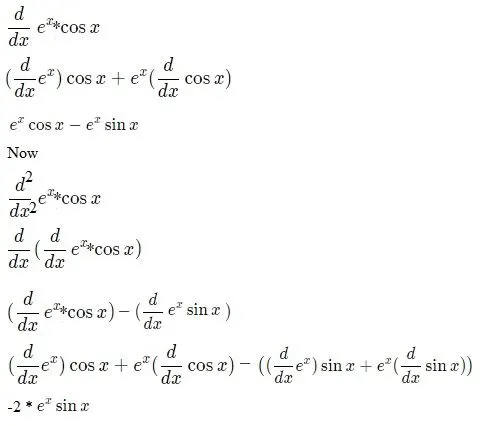
Analytical_Derivative = -2*exp(x)*sin(x)

Now we define our numeric deravitve using central diffrencing scheme as Central_Derivative

Now the syntex of our function defination has a varible out which give output value of function and now we define out is equal to error of our Numeric scheme.

The error is caluculate by abolute value of difference between Central_Derivative and Analytical_Derivative.

Now our code is

function out=Central_Differencing_Scheme(x,dx)
% Analytical function = exp(x)*cos(x);
% Analytical deravative = f'(x)= -2*exp(x)*sin(x);

Analytical_Deravative=-2*exp(x)*sin(x);

% Numerical derivative
% Central Differencing
% Coefficent value calculate in theory
a = -1/12;
b = 4/3;
c = -5/2;
d = 4/3 ;
e = -1/12 ;
% Central_Differencing=((a*f(x-2*dx))+(b*f(x-dx))+(c*f(x))+(d*f(x+dx))+(e*f(x+2*dx)))/(dx^2);
Central_Differencing=((a*exp(x-2*dx)*cos(x-2*dx))+(b*exp(x-dx)*cos(x-dx))+(c*exp(x)*cos(x))+(d*exp(x+dx)*cos(x+dx))+(e*exp(x+2*dx)*cos(x+2*dx)))/dx^2;

out=abs(Central_Differencing-Analytical_Deravative);
end

2) Function for Skewed right side differencing scheme of 4th order approximaation of second order derivatve of function exp(x)*cos(x)

Now we repete our previous processor but differenc is that we put our coefficent value claculated for our Skewed right side differencing scheme.

and we also define our numeric deravitve using Skewed right side differencing scheme as Skewed_Right_side_differencing

Now the syntex of our function defination has a varible out which give output value of function and now we define out is equal to error of our Numeric scheme.

then our code is

function out=Skewed_Right_side_scheme(x,dx)
% Analytical function = exp(x)*cos(x);
% Analytical deravative = f'(x)= -2*exp(x)*sin(x);

Analytical_deravative=-2*exp(x)*sin(x);

% Numerical derivative
% Right side skewe Differencing
% Coefficent value calculate in theory
a =15/4 ;
b =-77/6 ;
c =107/6 ;
d =-13;
e =61/12;
g = -5/6;
% Skewed_Right_side_differencing=((a*f(x))+(b*f(x+dx))+(c*f(x+2*dx))+(d*f(x+3*dx))+(e*f(x+4*dx))+(g*f(x+5*dx)))/(dx^2);
Skewed_Right_side_differencing=((a*exp(x)*cos(x))+(b*exp(x+dx)*cos(x+dx))+(c*exp(x+2*dx)*cos(x+2*dx))+(d*exp(x+3*dx)*cos(x+3*dx))+(e*exp(x+4*dx)*cos(x+4*dx))+(g*exp(x+5*dx)*cos(x+5*dx)))/(dx^2);

out=abs(Skewed_Right_side_differencing-Analytical_deravative);
end

3) Function for Skewed left side differencing scheme of 4th order approximaation of second order derivatve of function exp(x)*cos(x)

function out=Skewed_Left_side_scheme(x,dx)
% Analytical function = exp(x)*cos(x);
% Analytical deravative = f'(x)= -2*exp(x)*sin(x);

Analytical_deravative=-2*exp(x)*sin(x);

% Numerical derivative
% Left side skewe Differencing
% Coefficent value calculate in theory
a =-5/6 ;
b =61/12;
c =-13 ;
d =107/6 ;
e =-77/6 ;
g =15/4;
% Skewed_Left_side_differencing=((a*f(x-5*dx))+(b*f(x-4*dx))+(c*f(x-3*dx))+(d*f(x-2*dx))+(e*f(x-dx))+(g*f(x)))/(dx^2);
Skewed_Left_side_differencing=((a*exp(x-5*dx)*cos(x-5*dx))+(b*exp(x-4*dx)*cos(x-4*dx))+(c*exp(x-3*dx)*cos(x-3*dx))+(d*exp(x-2*dx)*cos(x-2*dx))+(e*exp(x-dx)*cos(x-dx))+(g*exp(x)*cos(x)))/(dx^2);

out=abs(Skewed_Left_side_differencing-Analytical_deravative);
end

Main program

• Now in the main program first we define value of x = pi/3. then we define a array dx using linspace inbilt function.Here line spacing makes an array of 20 indexing have data between pi/4000 to pi/4.
• Now we apply a for loop with increament i=1:length(dx).i.e. Loop is exicuted for each value of dx.
• In our loop we calculaed error of our Three Numeric schemes by calling their respective function for each value of dx.
• Now we plot the figure between dx(grid size) and error for each schemes and also plot logarithmic value by loglog funcion.
• we also calculating slope for each error at start and end value of dx.

% Numerical descreatization for 4th order approximation of 2nd order
% derivative
clear all
close all
clc
x=pi/3;
dx=linspace(pi/4000,pi/4,100)
for i=1:length(dx)
    dx(i);
    Central_Differencing_error(i)=Central_Differencing_Scheme(x,dx(i));
    Skewed_Right_side_differencing_error(i)=Skewed_Right_side_scheme(x,dx(i));
    Skewed_Left_side_differencing_error(i)=Skewed_Left_side_scheme(x,dx(i));  
end

figure(1)
plot(dx,Central_Differencing_error,'-o')
hold on
plot(dx,Skewed_Right_side_differencing_error,'-s')
plot(dx,Skewed_Left_side_differencing_error,'-d')
xlabel('log_dx');
ylabel('log_Error');
legend('Central Differencing Scheme','Right side skewed Differencing Scheme','Left side skewed Differencing Scheme')

figure(2)
loglog(dx,Central_Differencing_error,'-o')
hold on
loglog(dx,Skewed_Right_side_differencing_error,'-s')
loglog(dx,Skewed_Left_side_differencing_error,'-d')
xlabel('log_dx');
ylabel('log_Error');
legend('Central Differencing Scheme','Right side skewed Differencing Scheme','Left side skewed Differencing Scheme')



% Caluculating slope for initially ie for less step size
slope_Central_Differencing_Scheme=(Central_Differencing_error(2)-Central_Differencing_error(1))/(dx(2)-dx(1))
slope_Skewed_Right_side_scheme=(Skewed_Right_side_differencing_error(2)-Skewed_Right_side_differencing_error(1))/(dx(2)-dx(1))
slope_Skewed_Left_side_scheme=(Skewed_Left_side_differencing_error(2)-Skewed_Left_side_differencing_error(1))/(dx(2)-dx(1))

% Caluculating slope at end i.e. for larger step size
slope_Central_Differencing_Scheme=(Central_Differencing_error(100)-Central_Differencing_error(99))/(dx(100)-dx(99))
slope_Skewed_Right_side_scheme=(Skewed_Right_side_differencing_error(100)-Skewed_Right_side_differencing_error(99))/(dx(100)-dx(99))
slope_Skewed_Left_side_scheme=(Skewed_Left_side_differencing_error(100)-Skewed_Left_side_differencing_error(99))/(dx(100)-dx(99))

Result :- Now result in command window is

dx=.......... 100 values

and

slope_Central_Differencing_Scheme =

1.5932e-06

slope_Skewed_Right_side_scheme =

1.1509e-04

slope_Skewed_Left_side_scheme =

1.0346e-04

slope_Central_Differencing_Scheme =

0.4530

slope_Skewed_Right_side_scheme =

-43.8198

slope_Skewed_Left_side_scheme =

2.9643

Plots:-

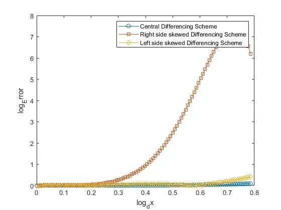
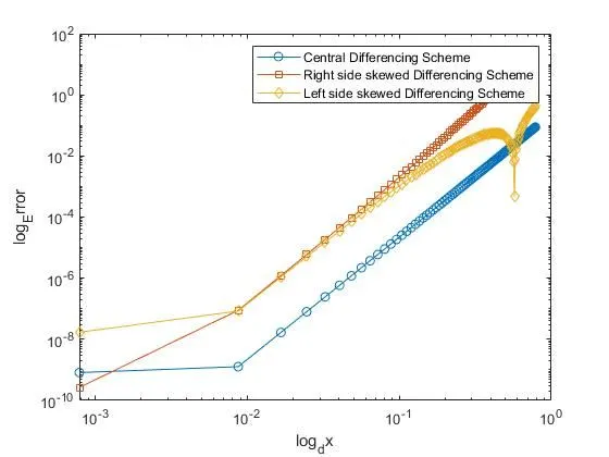
Note:-If here we don't use rational number of coefiicent values in our functions script then in our result log error is of 10^-3 at mesh size pi/4000 and in above graph it is between 10^-8 to 10^-10. so when we use irrational values there was error in result.so here above two graph are right and the below two graph are wrong.

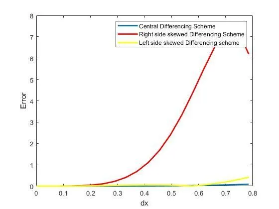
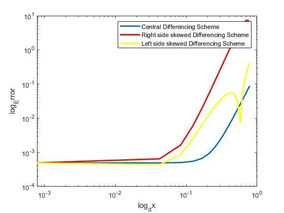
and if change our range of dx in main program pi/400 to pi/40 then our final result is

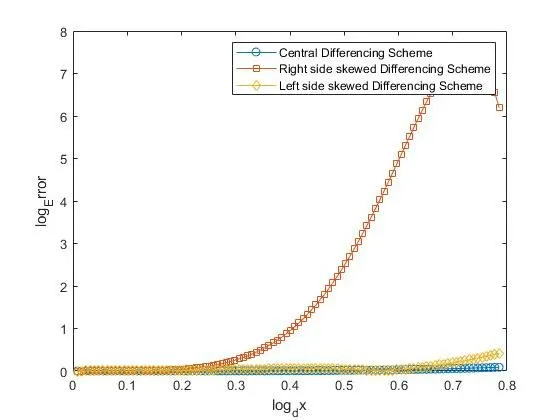
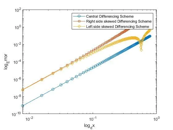
Here from above graph we observed that CDS have less error for each value of dx in range pi/400 to pi/40 in comparison to RSSDS. The log graph of LSSDS error is intially coinside on log RSSDS error graph but after some rang of dx it suddenly change ang go down to CDS error log graph and suddenly goes up.

Conclusion:- From the above graphs in result it is clear that CDS has less error compared to skewed schemes.from graph and result we also understand that the change in sploe of Right side skewed differencing scheme (RSSDS) more so we can accuracy drops faster in RSSDS as we inclerese the mesh size.

There for we can say that the Results in CDS is more accurate then other schemes because it take information from both side of our point of intrest to give numeric solution.

Here in above graph we also see that some higer value of dx or mesh size LSSDC have less error CDS.so we can use LSSDS for some lager step size where error is less.

Q.why a skewed scheme is useful? What can a skewed scheme do that a CD scheme cannot?

In our above study it was clear that CDS has more accurate solution then skewed schemes but sitll we use skewed schemes in some area where we don't have information from both side neighbouring points of considerations.

CDS can't use at boundares and corner points because of the absence of right or left side nodes.So at boundary node we use either right or left side skewed scheme instade of CDS.