Week 8 - Simulating Cyclone separator with Discrete Phase Modelling
Aim:- To perform analysis on cyclone separator and calculate the separation efficiency and pressure drop.
Objective:-
1. To perform an analysis on a given cyclone separator model by varying the particle diameter from 1 μm to 5 μm taking velocity at inlet 3m/s and calculate the separation efficiency in each case.
2. To perform an analysis on a given cyclone separator model by varying the particle velocity from 1 m/sec to 5 m/sec and calculate the separation efficiency and pressure drop in each case.
Theory:- A cyclone separator also known as cyclone dust collector is a devide use in chemical industries, coating industries for sparating micro particales present in fume gasses. This is also kind of dry scrubber.
A cyclone is a centrifugal separator in which particles, due to their mass, are pushed to the outer edges as a result of centrifugal force. Incoming air is automatically forced to adopt a fast-revolving spiral movement - the so-called “double vortex”. The dust and particle-laden air or gas enters the cylindrical chamber tangentially at one or more points and leaves through a central opening.
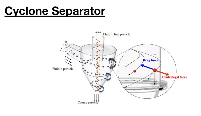
The size of the cyclone depends largely on how much flue gas must be filtered, thus larger operations tend to need larger cyclones. For example, several different models of one cyclone type can exist, and the sizes can range from a relatively small 1.2-1.5 meters tall.
Some smaller cyclone dust collector working on low CFM have exhaust fan at it's top and the larger CFM cyclone dust collector need ducting arrangmet with it.
Most cyclones are built to control and remove particulate matter that is larger than 10 micrometers in diameter. However, there do exist high-efficiency cyclones that are designed to be effective on particles as small as 2.5 micrometers. As well, these separators are not effective on extremely large particulate matter.
Separation efficiency:
It is defined as the fraction of particles of a given size collected in the cyclone, compared to those of that size going into the cyclone. Experience shows that the separation efficiency of cyclone separator increases with increasing particle mean diameter and density; increasing gas tangential velocity; decreasing cyclone diameter; increasing cyclone length; extraction of gas along with solids through the cyclone legs.
In this case, depending upon the particle history data - Separation Efficiency is defined as the ratio of concentration that has been removed from the feed stream to the initial concentration in the feed stream. For this case ratio of the number of trapped particles to the total number of particles tracked.
Separation efficiency = no. of particles trapped / no. of particles tracked
Pressure Drop:
Pressure drop across the cyclone is of much importance in a cyclone separator. The pressure drop significantly affects the performance parameters of a cyclone. The total pressure drop in a cyclone will be due to the entry and exit losses, and friction and kinetic energy losses in the cyclone. Normally the most significant pressure drop occurs in the body due to swirl and energy dissipation.
Pressure drop is defined as the difference in total pressure between two points of a fluid carrying netwon
Pressure drop, `Delta P` = Total inlet pressure - Total Outlet Pressure (escape)
Some emparical model for calculating seperation efficiency
The dimensions of the cyclones used in this study are given figure1
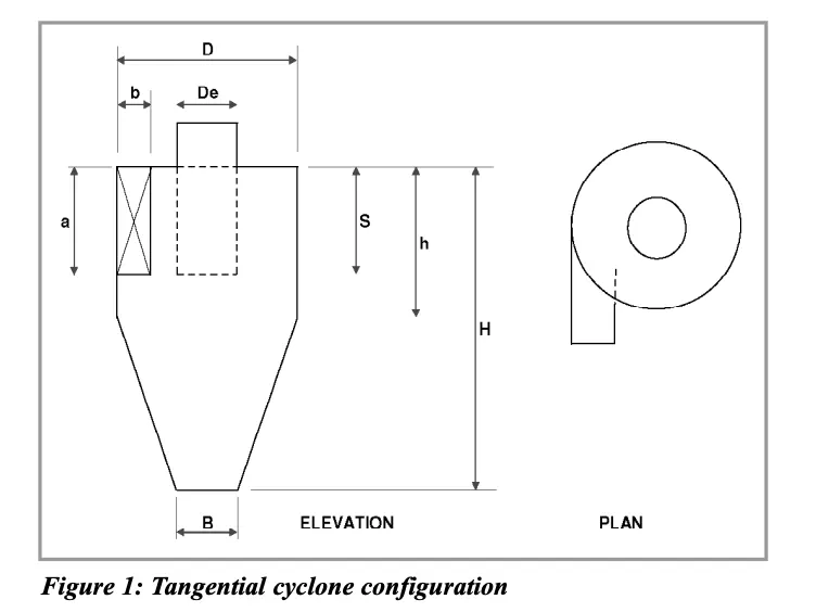
Here in our model these dimension are
H=800mm
h=400mm
b=50mm
a=100mm
De=100mm
D=200mm
B=50mm
S=250mm
IOZIA AND LEITH MODEL
Iozia and Leith (1990) logistic model is a modified version of Barth (1956) model which is developed based on force balance. The model assumes that a particle carried by the vortex endures the influence of two forces: a centrifugal force Z, and flow resistance, W. Core length, zc, and core diameter dc, are given as
`Z_c=(H-S)[(H-S)/((D/B)-1)][(d_c/B)-1]` For dc>B
`Z_c=H-S` For dc<B
`d_c=0.47(ab/D^2)^-0.25 (D_e/D)^1.4`
The addition made by Iozia and Leith on the original Barth (1956) model is the core length zc and slope parameter β expression which is derived based on the statistical analysis of experimental data of cyclone with D = 0.25 m. The collection efficiency ηi of particle diameter dpi can be calculated from
`eta_i=1/(1+(d_(pc)/d_(p i))^beta`
where dpc is the 50% cut size given by Barth (1956)
`d_(pc)=[(9muQ)/(piP_PZ_cV_max^2)]^0.5`
LI AND WANG MODEL
The Li and Wang (1989) model include particle bounce or re-entrainment and turbulent diffusion at the cyclone wall. A two-dimensional analytical expression of particle distribution in the cyclone is obtained. Li and Wang model was developed based on the following assumptions:
- The radial particle velocity and the radial concentration profile are not constant, for uncollected particles within the cyclones.
- Boundary conditions with the consideration of turbulent diffusion coefficient and particle bounce re-entrainment on the cyclone wall are:
`C=C_(P)` at`theta=0^*`
`D_r(delc)/(delr)=(1-alpha)w_c` at r=D/2
The tangential velocity is related to the radius of cyclone by: uRn = constant.
The concentration distribution in a cyclone is given as:
`C(r,theta)=(C_0(r_w-r_n)exp^((-lamda[1/(K(1+n))r^(1+n))]))/(int_(r_n)^(r_w) exp{1/(k(1+n))r^(1+n)}dr`
where
The resultant expression of the collection efficiency for particle of my size is given as
`K=((1-n)(rho_p-rho_g)d^2Q)/(18mub(r_w^(1-n)-r_n^(1-n))`
and
`lamda=((1-alpha)Kw_w)/(D_rr_w^n)`
ηi = 1 - exp {-λθ1}
where θ1 = 2π (S + L) / a
KOCH AND LICHT MODEL:-
Koch and Licht (1977) collection theory recognized the inherently turbulent nature of cyclones and the distribution of gas residence times within the cyclone. Koch and Licht
describe particle motion in the entry and collection regions with the additional following assumptions:
- The tangential velocity of a particle is equal to the tangential velocity of the gas flow, i.e. there is no slip in the tangential direction between the particle and the gas.
- The tangential velocity is related to the radius of cyclone by uRn=constant">uR^n=constant
A force balance and an equation on the particle collection yields the grade efficiency ηi
`eta_i=1-exp{-2[G tau_iQ/D^3(n+1)]^(0.5(n+1)}`
where
`G=(8K_e)/(K_n^2 K_b^2)`
`n=1-{1-(12D)^0.14/2.5}{(T+460)/530}^0.3`
`tau_i=(rho_pd^2)/(18mu)`
G is a factor related to the configuration of the cyclone, n is related to the vortex and τ is the relaxation term.
LAPPLE MODEL:-
Lapple (1951) model was developed based on force balance without considering the flow resistance. Lapple assumed that a particle entering the cyclone is evenly distributed across the inlet opening. The particle that travels from inlet half-width to the wall in the cyclone is collected with 50% efficiency. The semi-empirical relationship developed by Lapple (1951) to
calculate a 50% cut diameter, dpc is
`d_(pc)=[(9mub)/(2piN_eV_i(rho_p-v_g))]^(1/2)`
where N is revolution
`N=1/a[h+(H-h)/2]`
`eta_i=1/(1+(d_(pc)/d_(pi))^2)`
Referance:-The above data is taken from http://dspace.unimap.edu.my/bitstream/handle/123456789/13571/054-058_empirical%20models.pdf?sequence=1&isAllowed=y#:~:text=It%20appears%20that%20the%20Lapple,reasonable%20prediction%20under%20these%20conditions.
Simulation process
1) Pre processing
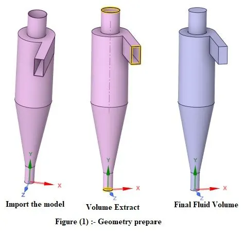
a) Modeling:- First we import the model in Ansys fluent and then go to prepare and extract the fluid volume by selecting the boundary edges. Then supress mode for physics and hide it only fluid volume is remain.
b) Meshing :- Now close the space claim and open the mesh module, Now go to method and define Cartesian and give element size 5mm then generate mesh.
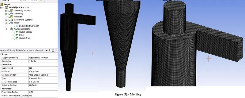
Naming the boundaries
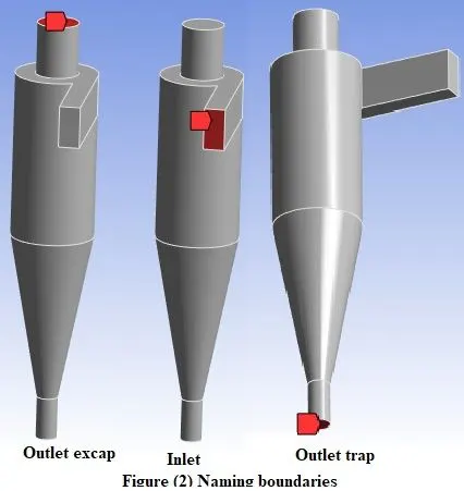
2) Analysis Setup:- Now open Ansys fluent
General setup
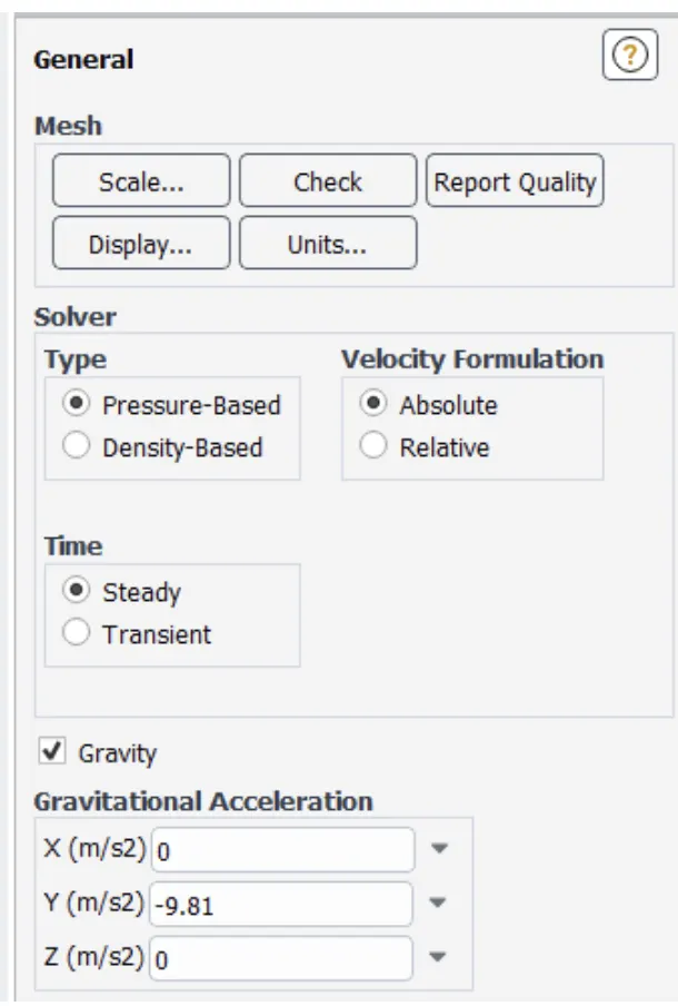
Here we use pressure base slover and Steady state analysis with gravity 9.81m/s2 in -ve Y direction
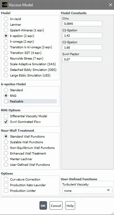
Viscous model :- Here we choose k-epsslion RNG model with Swril dominated flow in RNG option because in cyclone there is swril flow. and also use standerd wall function.
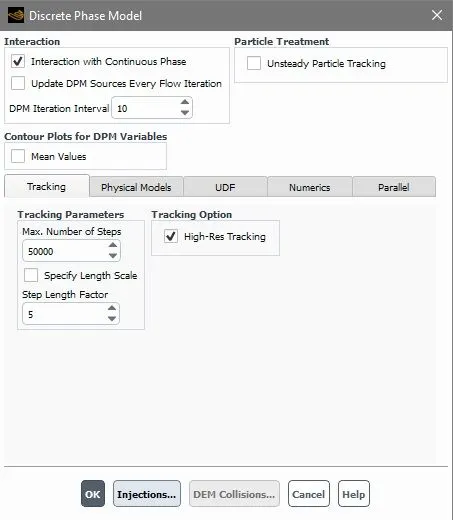
Discrete phase model:- In ansys fluent we use langragien discrete phase model which is similar to elurien approach for fluid dynamic study in which we study behviour of each partical. This DPM is can solve continuty , momentum and energy equastion.
Here in ansys there are two catogary of DPM 1) coupuled and 2) uncoupled
In Uncoupled the discrete phase phase not have any interaction with continuous space. where as coupled discrete phase will influence the flow with continuous space but the size of partical injected in cyclone seperator is very small.
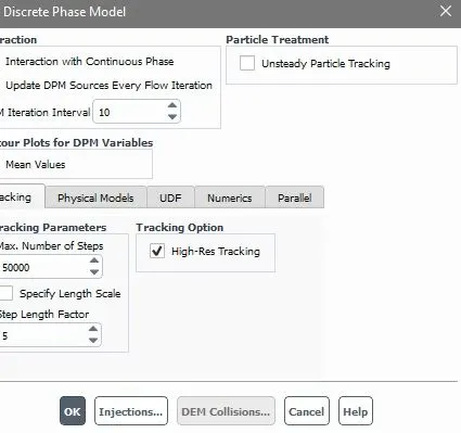
now click on ijection to give the setting
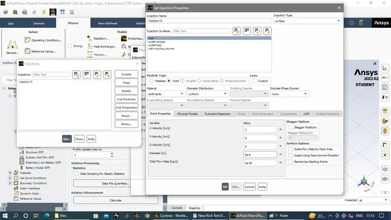
Now give material as anthracecite and injection at inlet
Now you can give velocity and diameter size Here you can paramereize either one of them or both.
Boundary condition
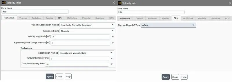
Now also give inlet velocity at boundary condition and if we paramererize velocity at DPM we have also paramererize velocity in boundary condition.
Here in DPM choose reflect type.
Solution Method
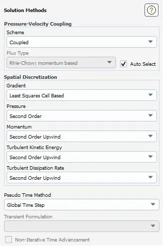
Here first we choose coupled scheme for pressure velocity coupling
an dthen in special descretization of pressure is second order and for momentum, turbulent K.E and dissipation rate this is second order upwind .
Run analysis
Now run the alalysis at 250 iteration with Hybrid initilazation.
now after completing alalysis we we have to export the partical data
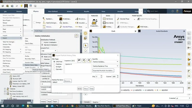
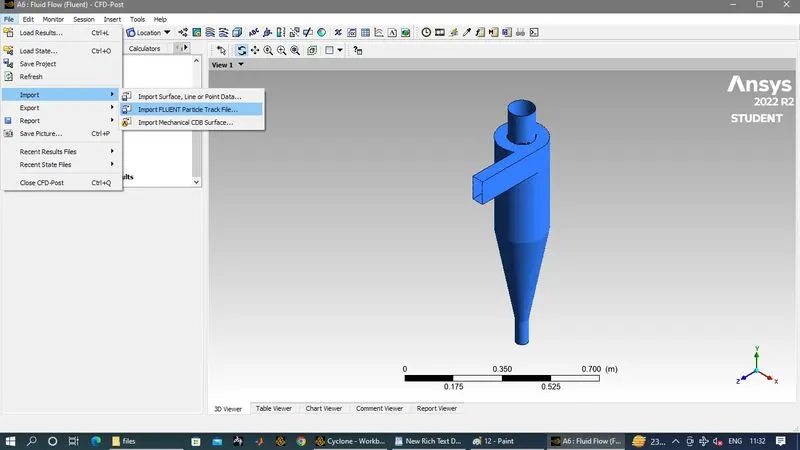
3) Post procedure:- Now close fluent and open CFD post and import the partical track file
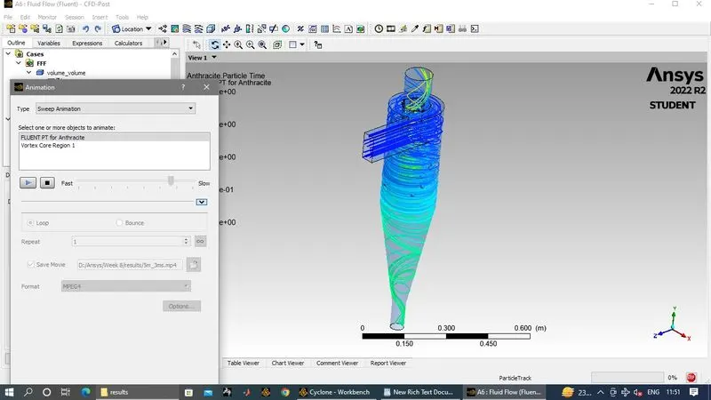
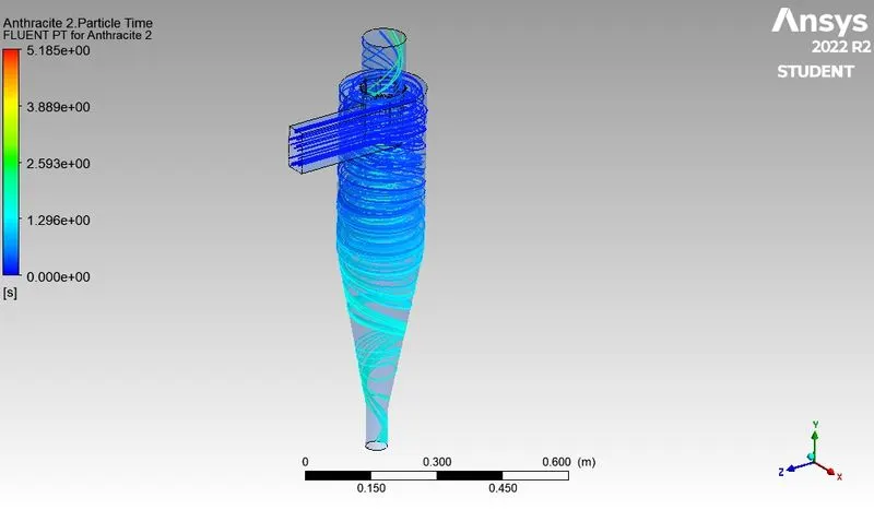
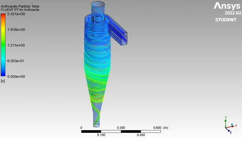
now tincrease tranpriency of cyclone wall and give render varible to Anthercite partical time and for animation go to animation create animation for one loop.
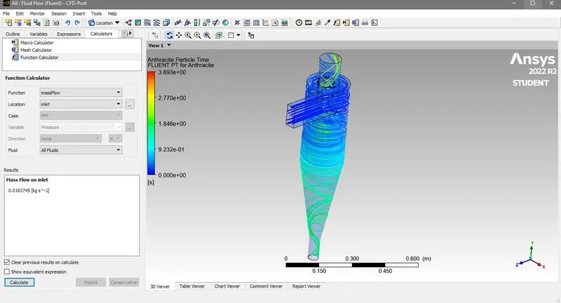
Now here we can calculate mass flow rate and pressure at inlet and outlet
Case study
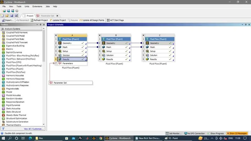
1) Our first study is by varying the particle velocity from 1 m/sec to 5 m/sec for partical size 5 micron. Here in ansys work bench first i drag a fluent module and
do above steps, only change is i makes velocity as parameter at both side either inlet boundary condition or in DPM also. Now varing this velocity i perform an parametric study of three design point
Dp0==> velocity is 5m/s
Dp1==>velocity is 3 m/s
Dp2==>velocity is 1 m/s
2) Our second study is by varying the partical size 1micron to 5 micron at velocity 3m/s. So here i creates two more fluent study and copy geomety and mesh data as shown in figure
Result:-So finaly i have these five studies which results are conconsole when writing partical data and also pressure at inlet and outlet escap are
Case1.1 Partical size 5 micron and velocity 1m/s
Total pressure at inlet =31.93053 pa
Total pressure at outlet escap=10.78732 pa
number tracked = 378, escaped = 134, trapped = 244
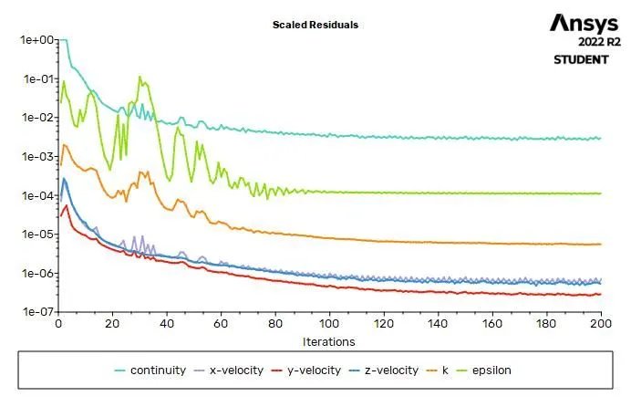
Residual plot
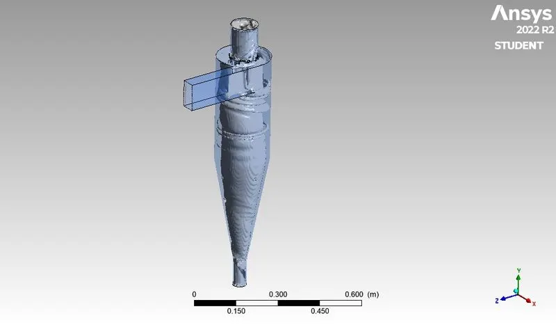
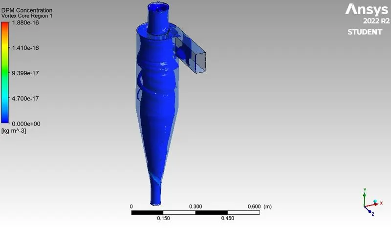
Vortex
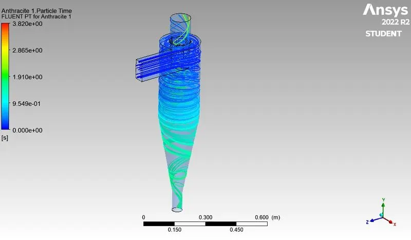
Partical Time
Animation
Case1.2 Partical size 5 micron and velocity 3m/s
Total pressure at inlet =31.9161 pa
Total pressure at outlet escap=10.78269 pa
number tracked = 378, escaped = 130, trapped = 248
Residual plot
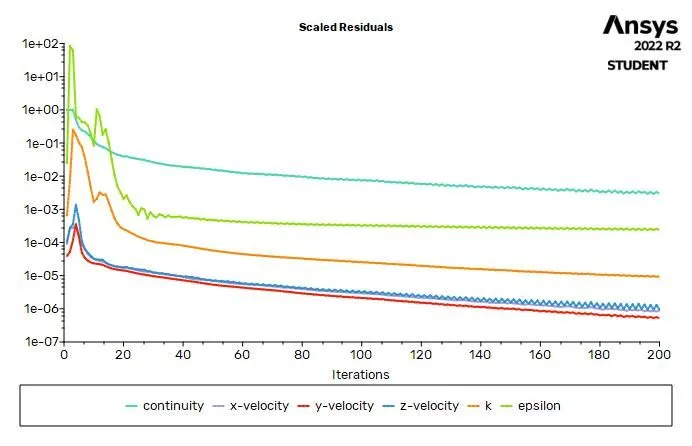
Vortex
Partical Time
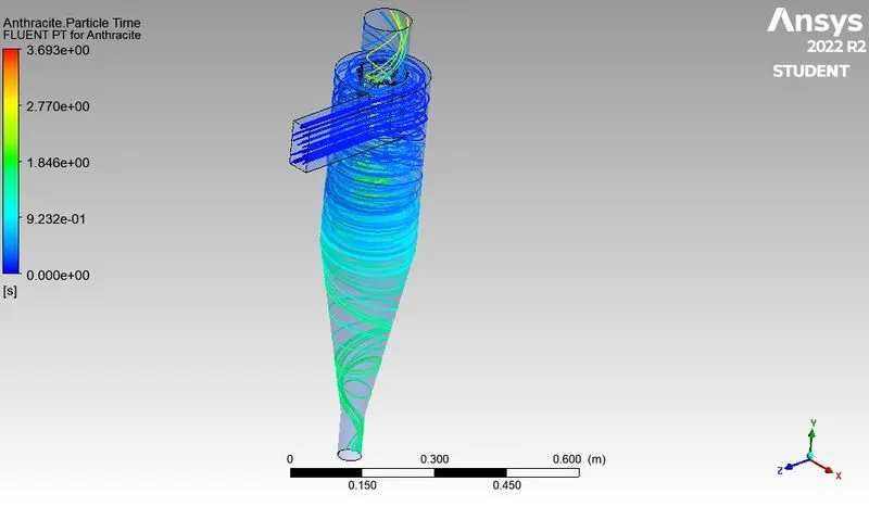
Animation
Case1.2 Partical size 5 micron and velocity 5m/s
Total pressure at inlet =31.92948 pa
Total pressure at outlet escap=10.78656 pa
number tracked = 378, escaped = 132, trapped = 246
Residual plot
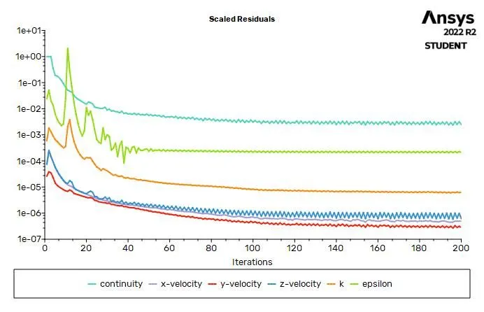
Vortex
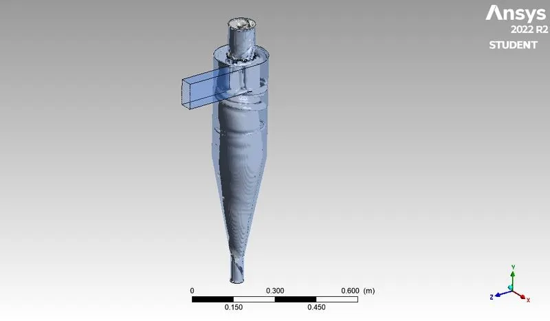
Partical Time
Animation
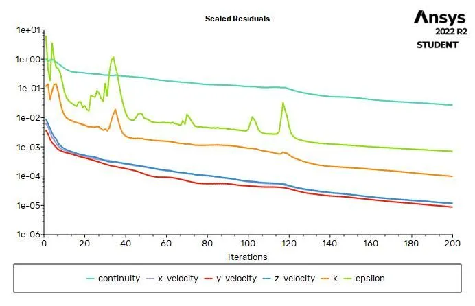
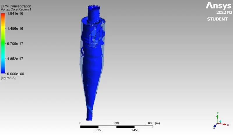
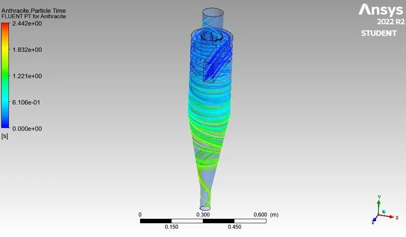
Case2 Partical size 3 micron and velocity 3m/s
Total pressure at inlet =31.18816 pa
Total pressure at outlet escap=4.298285pa
number tracked = 378, escaped = 70, trapped = 30822
Residual plot
Vortex
Partical Time
Abimation
Case3 Partical size 1 micron and velocity 3m/s
Total pressure at inlet =31.18816 pa
Total pressure at outlet escap=4.298285pa
number tracked = 378, escaped = 73, trapped = 305
Residual plot
Vortex
Partical Time
Animation
Tabuler data from result calculation
| Partical Size | Velocity | △p (pa) | Parical Tracked | Partical Traped | Efficincy By Lapped model | Efficincy by simulation |
| 5 micron | 1m/sec | 21.1432 | 378 | 244 | 99.46% | 64.55% |
| 5 micron | 3m/sec | 21.1334 | 378 | 248 | 99.94% | 65.60% |
| 5 micron | 5m/sec | 21.1329 | 378 | 246 | 99.97% | 65.07% |
| 3 micron | 3m/sec | 26.8898 | 378 | 308 | 99.94% | 81.48% |
| 1 micron | 3m/src | 26.8899 | 378 | 305 | 98.53% | 80.68% |
Conclusion
- From above tabuler data we can obereved that pressure dropes at ecape is constant for constant parical size 5 micron, so we conclude that it depents upon partical size.
- There parical traped are more when we reduce paritical size so the efficiency depends on the parical size.
- The seperation efficiency depends on parical size, design of cyclone and CFM of exhaust fan ect.
- As the size of the particle decreases and the velocity of the flow decreases, the time is taken for convergence also increases. So to overcome this, the maximum no of steps in tracking parameters are increased.