Week 5 - Rayleigh Taylor Instability

Aim:- To simulate Rayleigh Taylor Instability in Ansys Fluent.

Introduction:- Rayleigh Taylor Instability is a phenomenon that occurs at interface of two fluids of different density where intialy heigher density fluid put on upper side of lighter fluid and saperetes by a plate as we remove plate higher fluid move down due to gravity and lighter fluid go up by buoyancy forces and a pattern of continues up and down moment is develope untill the comes in the equllibrim states.

When we remove the plate intialy what havppent at interface, the havier particals tends to go downward due to gravity and lighter particals tends to move upward due to pressure and this upward and downdard moments of particals ripple in the surface dividing liquids will grow because of higher potential energy of tota system (combine of both fluid) and this stage is called unstable state.

After this initally this instability is increases and developing plums (upward movement) and spikes (downward movement) with the time, after some these time the amplitude of these plums and spikes is reducing with time because of reduction in potential energy of particals untill the equllibrim state.

some example of this are

1. singel fluid model of two different phase:- water and water vapour.

2. multi fluid model of single phase:- gases like Co2 in air, smoke in air.

3. multi fluid model of different phase: air and water.

4. adibatic mixing of two gause and fluid.

5. Plasma and vaccume

Practical CFD models that have been based on mathematical analysis of Rayleigh wave

1. Kelvin-Helmholtz instability
2. Richtmyer-Meshkov instability
3. Plateau-Rayleigh instability

Kelvin-Helmholtz instability- This instability typically occurs when there is velocity shear in a single continuous fluid, or additionally where there is a velocity difference across the interface between two fluids. A common example is seen when wind blows across a water surface; the instability constant is able to manifest itself through waves on water surface. The Kelvin-Helmholtz instability is not only restricted to a water surface as clouds, but is evident through other natural phenomena as ocean and the sun's corona.

Richtmyer-Meshkov instability- This occurs when two fluids of different density are impulsively accelerated. Normally this is by the passage of a shock wave. The development of the instability begins with small amplitude perturbations which initially grow linearly with time. This is followed by a nonlinear regime with bubbles appearing in the case of a light fluid penetrating a heavy fluid, and with spikes appearing in the case of a heavy fluid penetrating a light fluid. A chaotic regime eventually is reached and the two fluids mix. This instability can be considered the impulsive-acceleration limit of the Rayleigh Taylor instability.

Plateau-Rayleigh instability- This instability, often just called the Rayleigh instability, explains why and how a falling stream of fluid breaks up into smaller packets with the same volume but less surface area. It is related to the RTI and is part of a greater branch of fluid dynamics concerned with fluid thread breakup. This fluid instability is exploited in the design of a particular type of ink jet technology whereby a jet of liquid is perturbed into a steady stream of droplets. The driving force of the Plateau–Rayleigh instability is that liquids, by virtue of their surface tension, tend to minimize their surface area.

Procdure:-

Pre processing

Step1:-Preparation of Geometry

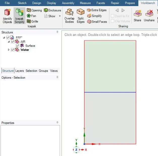
First open Ansys Spaceclaim and go to sketcher and select the xy plate as shown in image and then create rectange of 20x20 mm2 from origion point.Now exit sketcher by clicking press pull and select surface right click and click new componet name air. now click on right new model name water go to sketch create another recatangle of 20x20 above the privious rectangle.

Here now we active share topology between these to componet.

Step2:- Mesh Generation

Now come to mesher environment and simple generates the mesh. Here ansys by defult generates hex mesh and this is simple 2d geometry so mesh quality also good.

here we have three case

1st is water and air with elemnet size 0.5mm

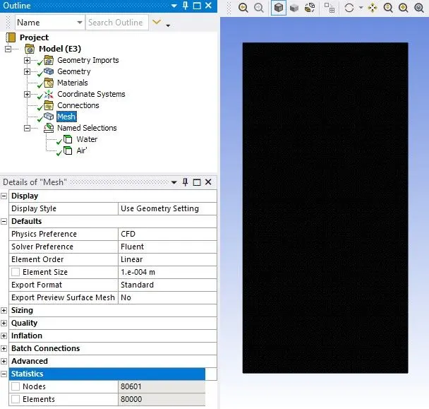
2nd is water and air with element size 0.1mm

and 3rd case is user define fluid with air and element side 0.1mm

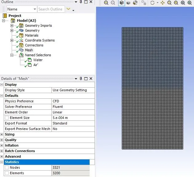
and the refine mesh are

Then we naming the region as water and air and close the mesher environment.

3 Setup

now open fluent by double click setup

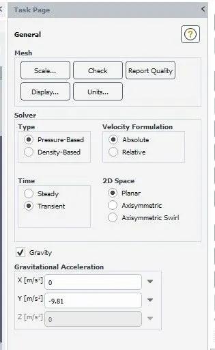
Here we choose pressure base solver because here flow in incompressible. and i choose Transient analysis because i have to study how to fluid mixed and comes to equiilbrim with respect to time or check how Raleigh wave is develope and stable with respect to time.

Here i Active the gravity and give gravitational acceleration is qualt to 9.81m/s2 in -ve y direction.

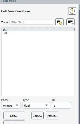
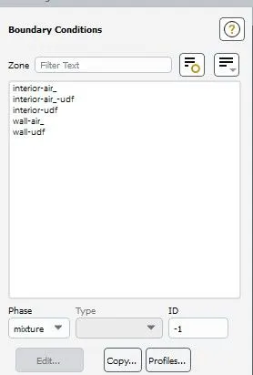
Now come to cell zone and see air and water or UDF (in case 3) cells here phase of these is mixture.

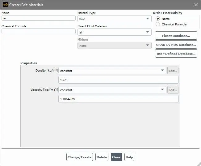
Now came to material select the air as defult properties in fluent. and choose water with defult properties.

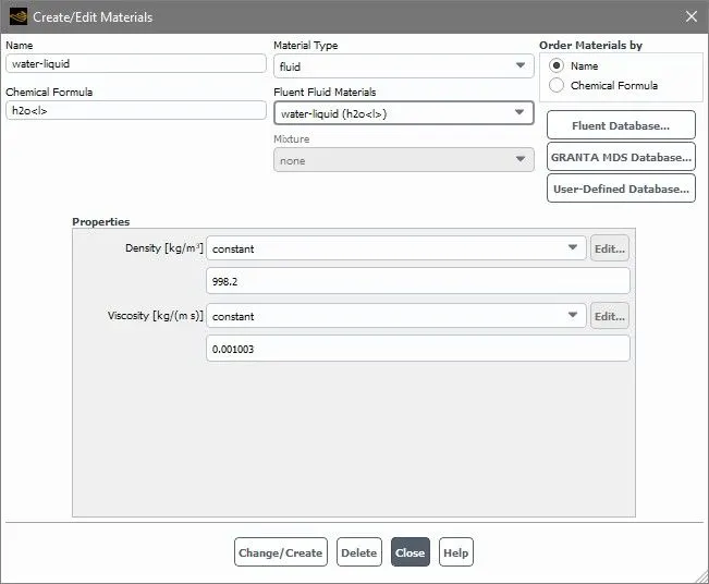
Now for case 3 we have to select a different material. so first click on Fluent database copy Water-liquid(h20<1>)and paste with new name udf.

change it desity to 400kg/m3 and viscosity 0.001kg/ms.

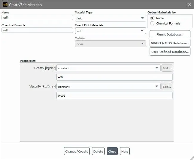
Model selection

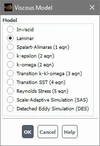
Now in Viscous model select the laminar because here turbulance eddies are occures in simulation but still flow velocity is less and flow is consider as laminar.

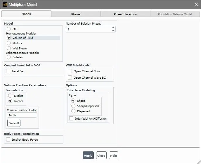
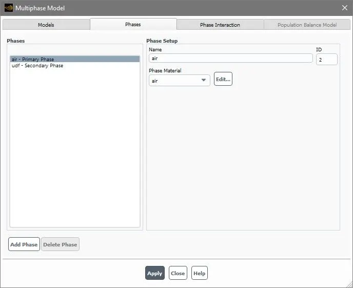
Now here we have to go multiphase model select model as Volume of Fluid and in volume fraction parameters select the Implicit formulation.Select the number of phase 2 and come to phase and here assine phase material for air and water or udf (in case 3).

Patching

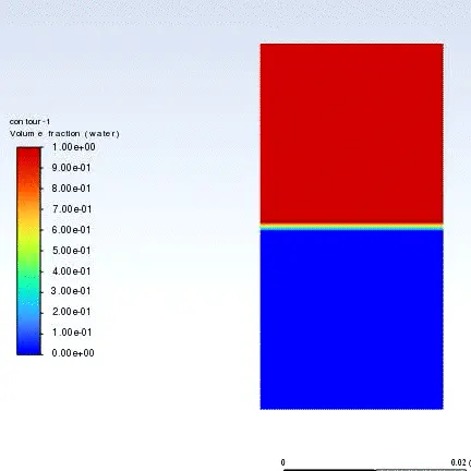
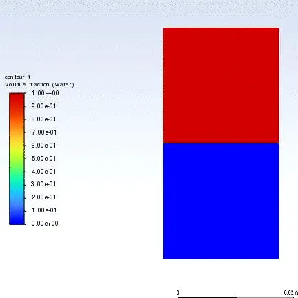
here we define this which phase matrial in which region in initial state by defining fraction of water in the both of the region. In air region volume fraction of water is 0 and in water region volume fraction is 1.

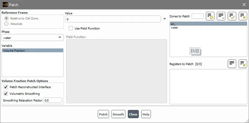
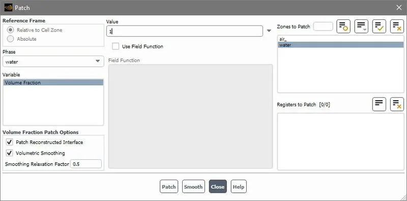
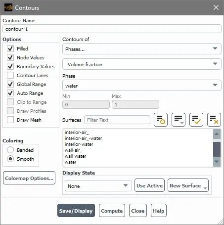
Here we are defineing legands of contour plot also because our legend is volume fraction of water changing in the simulation.

Now come to contour plots and select contours of phase , volume fraction of water phase or udf.

Run time setting

For case 1. Here as my analysis is transient so i have to choose time step size in shuch a way CFL number is less then 0.5 becuase model is 2d.

so my time step size is 0.005 sec and number of time step is 1000.

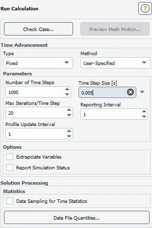
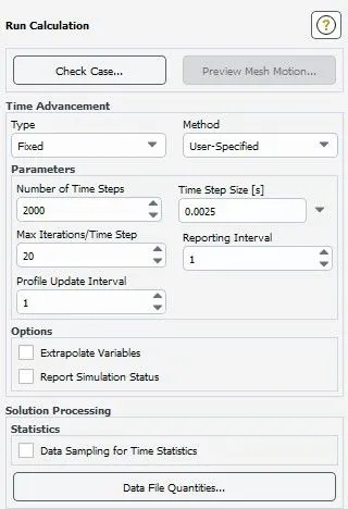
for case 2 and 3 mesh is fine so for stability i choose time step size 0.0025 sec and number of time step is 2000 for maintaining flow time same in both case.

because flow time = time step size in sec x number of time step =0.005*1000= 5sec and 0.0025*2000= 5 sec

Now run the analysis.

Simulatio result

Case1 (water and air with mesh size 0.5mm)

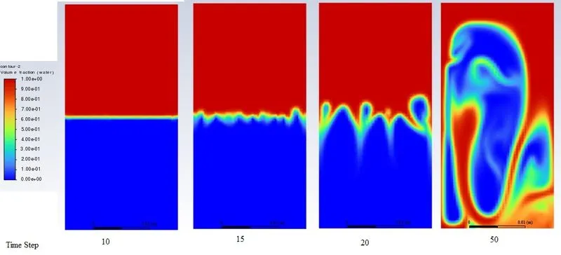
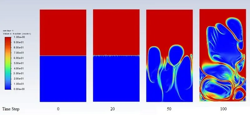
Now here in the above image you can see how particales are moving or transfering at interface in intial time step. and how plums and spikes are developes near to the inrerface at time step 20 and how their aplitude is increase in time step 50.

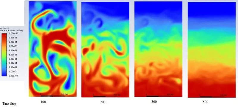
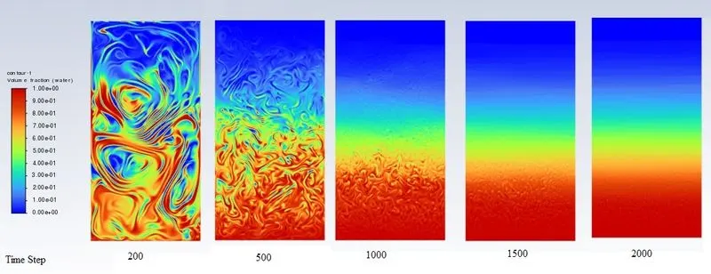
After the 100 time step the amplitude of this twisting pattern is reducing and at end of 500 time you can see clouds of mixture as shown in figure

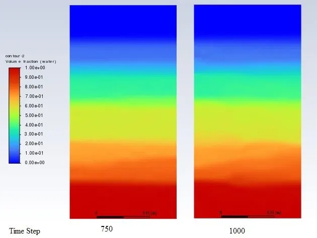
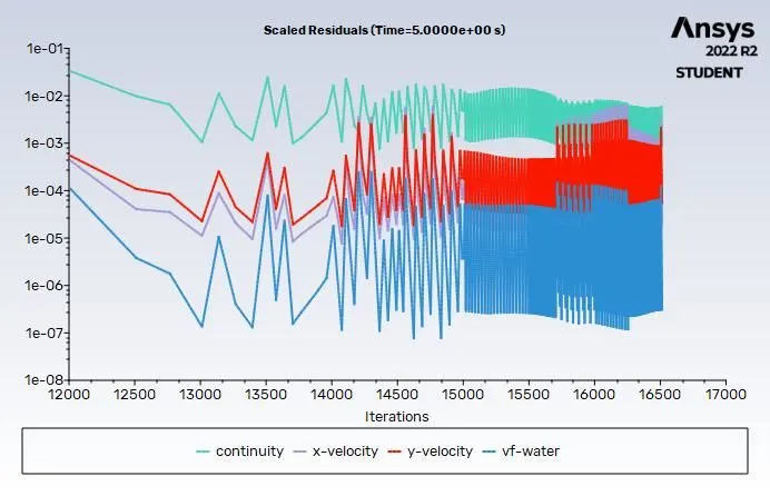
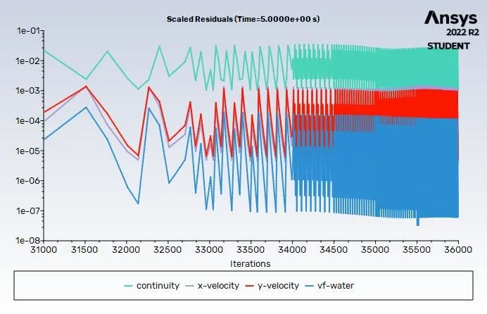
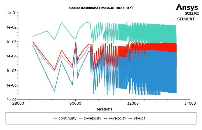
The solution is conveger after 1000 time step or 5 sec flow time. Residual plot

Solution animation

Case2 (water and air with mesh size 0.1mm)

Here you can see eddy developement in simulation are grow with time step 1 to 100 like privious case but here eddies pattern are smoother then privour case because of fine mesh but it take more run time.

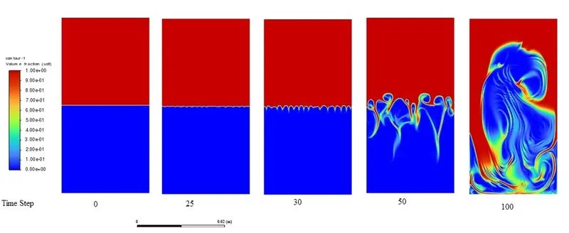
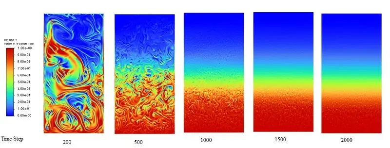
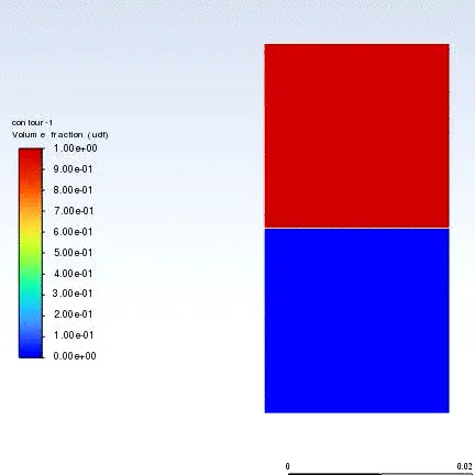
Case3 (air with user define fluid having desity 400kg/m3)

Atwood Number

It is a dimensionaless number that is used to study hydrodynamic instabilities in density stratified flows.

A=`(rho_1-rho_2)/(rho_1+rho_2)`

where

ρ1 is density of heavier fluid

ρ2 is density of lighter fluid

For Air water mixture it value is 0.998 (For case 1 and 2) and for case 3 (water with fluid density 400kg/m3) it valve is calculeded as 0.428.

Result summery of all above case simulation

1. and these bubbles formeres almost after 1000 time step which show that at the time where mixture come to equllibrim in case1 but in case2 it is still showing Rayleigh instability.
2. If we see all three case of Rayleigh instability which envolves first boundary mixing ,Mushroom head falling , eddies formation, bubble formation and merging of mixture. and if understand Atwood number with these case study for low Atwood number (i.e. case 3) the bubble and mushroom head shape are symmetrical,and the distrubance are linear for a larger time but for large atwood number (i.e. case 1 and 2) bubble and mushroom head shape are less symmetrical and also occure very rapidly at an accelerating rates which leads to a non linear groth.

Conclusion:-

• In CFD Rayleigh instability phenomina can be capture more effectively by using Fine mesh as compare to coare mesh But fine mesh model take more time to give result .
• Since this type of simulation involves capturing instabilites that is changing in an unpredictable manner as a function of time,the transient approach is preffered.
• The Atwood Number ,which is ratio of density difference and it's is responsible for behaviour of mixing and formation of bubbkes.