Week 1- Mixing Tee

Aim:-To study mixing effectiveness of a short and long mixing tee for different momentum ratio with CFD analysis in Ansys Fluent.

Theory:- Mixing Tee is a unit use in Thermal engineering cycles (like petrochemical, HVAC ) where two fluid of different states or phases are mixing and go to another units. For example an airconditioning plant in which conditioned air (at room temperature) is mixing with fresh air coming from outside (at ambiant temp.) to maintain air quality and Temperature inside the room. The effectiveness of mixing tee is define as uniformity of mixing at outlet of tee.

Now in this challange we have give two CAD models of mixing tee, having diffrence in there length only and we have to performe CFD simulation in steady-state at two different momentum ratio 2 & 4.

Momentum ratio=Velocity of inlet cold fluid / Velocity of inlet hot fluid

`M_r=V_c/V_h`

Given data is

Temperature at inlet cold fluid =19℃

Temperature at inlet hot fluid =36℃

Now here we have four cases

case -A (Long mixing tee Model)

• Hot inlet velocity of 3m/s.
• Cold inlet velocity of 6m/s. (because Momentum ratio is 2)

case -B (Long mixing tee Model)

• Hot inlet velocity of 3m/s.
• Cold inlet velocity of 12m/s. (because Momentum ratio is 4)

case -C (Short mixing tee Model)

• Hot inlet velocity of 3m/s.
• Cold inlet velocity of 6m/s. (because Momentum ratio is 2)

case -D (Short mixing tee Model)

• Hot inlet velocity of 3m/s.
• Cold inlet velocity of 12m/s. (because Momentum ratio is 4)

we have to simulate these case and evaluate result with analytical solution using below formula derived by appling energy and mass balance equastion

`m_c^.+m_h^.=m_o^.`

`V_o=V_h+V_c[d_c/d]`

here `d_c= diameter of cold inlet duct`and d=diameter of hot inlet and outlet duct

`T_o=(m_c^.T_c+m_h^.T_h)/m_o^.`

Now in mixing tube there is Turbulance flow with flow separation.In Turbulance flow there is two compnets of velocites

average compnet of velcity and the fluctuating component of velocity

now in our Navior strock equastion `sumF=ma⃗`

`rhodV[u(du)/dx+v(du)/dy+w(du)/dz]=-(delrho)/dx dV+mu[(del^2u)/dx^2+(del^2u)/dy^2+(del^2u)/dz^2]`

In the turbulance flow due to the fluctuating component of velocity there is existing Reynolds stress.

`sigma_(ij)^'=[[(sigma_(x x)^',tau_(xy)^',tau_(xz)^')] ,[(tau_(yx)^',sigma_(yy)^',tau_(yz)^')],[(tau_(zx)^',tau_(zy)^',sigma_(zz)^')] ]`

where `tau_(xy)^'=rho(u'v')` and `sigma_(xx)^'=rhou'^2`

Now adding thisReynolds stress in Navior strock equastion we get Reynolds average Navior strock equastion which is very importand equastion for turbulance model.

There two most important model for turbulance SST simulation

(1) K-epsilon (k-ε) turbulence model is the most common model used in CFD to simulate mean flow characteristics for turbulence flow conditions. It is a two equation model that gives a general description of turbulence by means of two PDEs.k-ε model focuses on the mechanisms that affect the turbulent kinetic energy.The underlying assumption of this model is that the turbulent viscosity is isentropic, in other words, the ratio between Reynolds stress and mean rate of deformation is the same in all directions.

k is turbulance kinetic energy and ε is rate of dissipation of the turbulence kinetic energy k into internal thermal energy

The k-ε model has been tailored specifically for plane shear layers and recirculating flows. This model is the most widely used and validated turbulance model with applications ranging from industrial to environmental flows, which explains its popularity. It is usually useful for free-shear layer flows with relatively small pressure gradients as well as in confined flows where the Reynolds stress are most important.

However it is more expensive because of two extra PDEs solve requred more mamory. The k-ε model also performs poorly in a variety of important cases such as unconfined flows , curved boundary layers , rotating flows in non circulating ducts.

Limitations of k -epsilon
-No-slip walls
-Adverse pressure gradients
-Strong curvatures
-Jet flows
-Difficulty solving for epsilon

(2) k-omega(k–ω) turbulence model is use an approximation of Reynolds average Navior strock equastion. the model attempts to pridict turbulence by two PDEs for two varible K and ω.

k is turbulance kinetic energy and ω is specific rate of dissipation of the turbulence kinetic energy k into internal thermal energy

This model not required wall function so low memory requirement. but it is inaccurate for adverse pressure gradient , strong curvature, and jet flow.

Limitations of k -omega
-Difficulty of convergence compared to k -epsilon
-Sensitivity to initial conditions

here in this case we use k-ε model because it is recirculating flow.

Procdure:- First open the Ansys workbench and drage the Fluid Flow (Fluent) from toolbox to project scemaric window as show in below image.

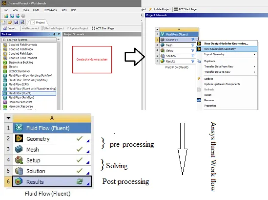
Now from above image we can understand the work flow of ansys Fluent so right click to gemetry and open Spaceclame Geometry.

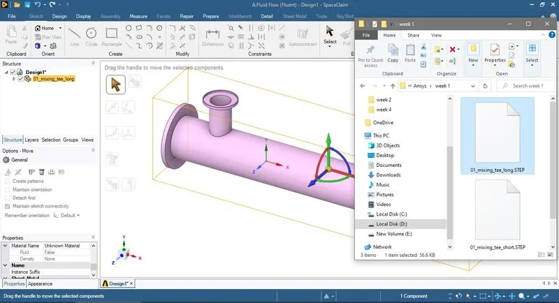
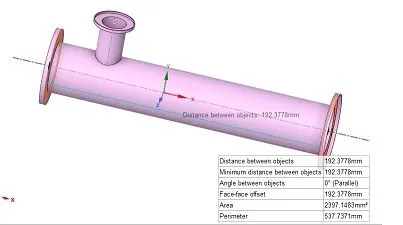
Now in Spaceclame check the units of model and measure the model

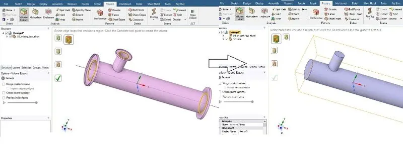
Here in Spaceclame we only need to extract the volume so go to the Prepare tab click on Volume Extract ribbon. and click edge selection and select the free edges of mixing tee

Now close the spaceclaim.

(2) Meshing :- Now double click on mesh and mesh enviroment is open. Now in project Outline at left side of window expand the Model tree click on Mesh.

Now in Details of "Mesh" you cad define Element Size equal to 0.2m. Now click on Generate in mesh ribbon.

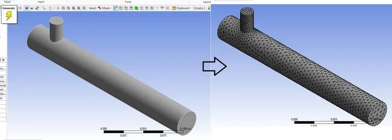
Now here type of Mesh is defult we can change by right click mesh >Insert >Method and select any method from list given.here i choose defult mesh type.

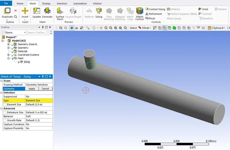
Now here the joining edge of tee duct is critical region so i am refining this by Sizing.

> Insert>Sizing. Now select edge from selection filter and select the joining edge of tee ducts.

Now go to Details of "Edge Sizing" in Defination select Number of division as Type and give value 50 which is best sutable value for given model for element size 0.2m.

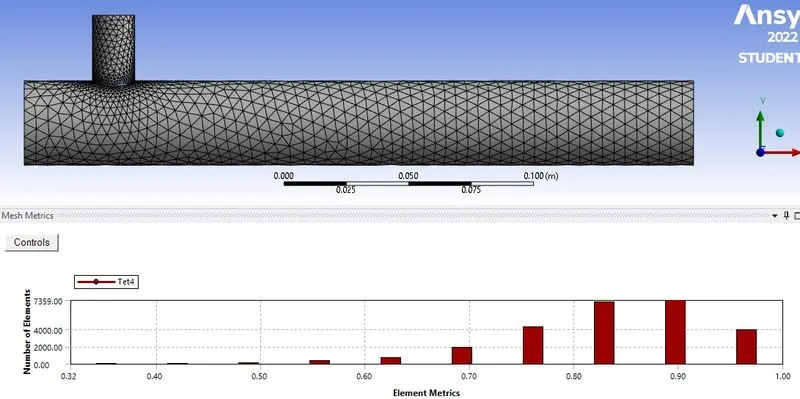
now again generates mesh and then go to qulites select Number of elements to check mesh quality

(3) Naming Boundaries :- Now in mesh enviroment select face in selecting filter and Select faces of tee geometry assime their boundaries by pressing N.

the boundaries are

Inlet-x (inlent of hot fluid)

Inlet-y (inlet of cold fluid)

Outlet (outlet of mixture)

Wall (stationary walls of tee ducts)

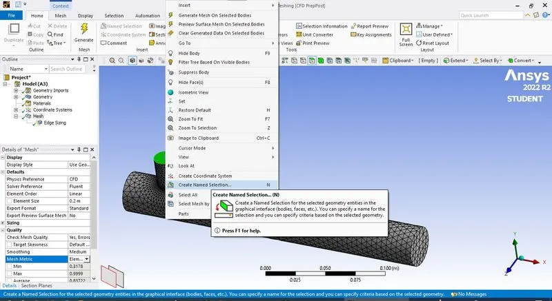
Now our pre-processing is done now come to solve part exit the mesh enviroment.

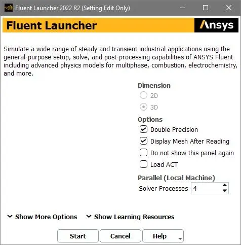
(4) Setup :- Now double click the setup to open setup mode, firts it open Fluent Launcher where we can edit solver setting check Double Precision and Select Parallel solver with processes 4 and click Start button.

Now Ansys fluent solver enviroment is open first go to Domain Tab click Check ribbon to check mesh of geometry.

Now go to Physics Tab select Solver Type Pressure-Bassed and Velocity Formulation is Aboslute.

and then select Steady for steady state solution and check Energy to active calculation with energry equastion.

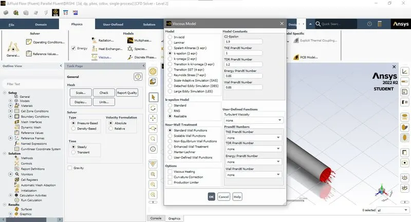
Now Select Viscous Model and select the k-epsilon model and click ok.

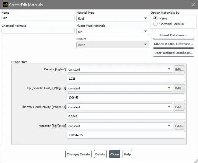
Now click material to edith material here defulat material is allready given so click ok.

(5) Assining Boundary condition:- Ansys automaticaly assine the boundaries which we name in Mesh enviroment we only have to give boundary conditions on these bondaries. Before this i change my units by clicking units.

Now expan setup tree expand Boundary conditions in inlet click Inlet-x and define velocity 3 m/s. and go thermal and define temperature 36℃.

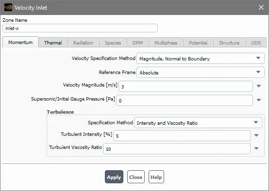
now click Inlet-y define velocity 6m/s and temperature 19℃.

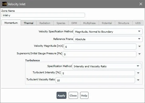
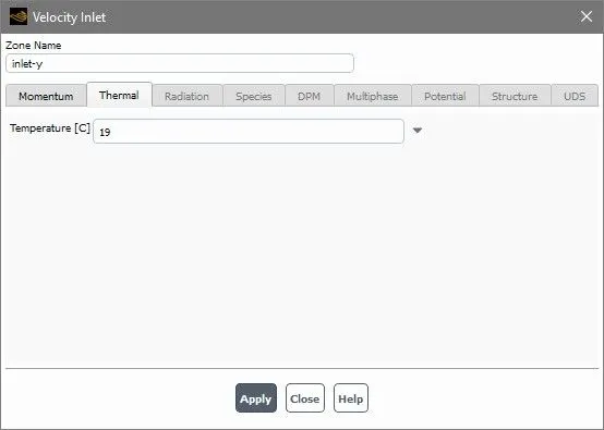
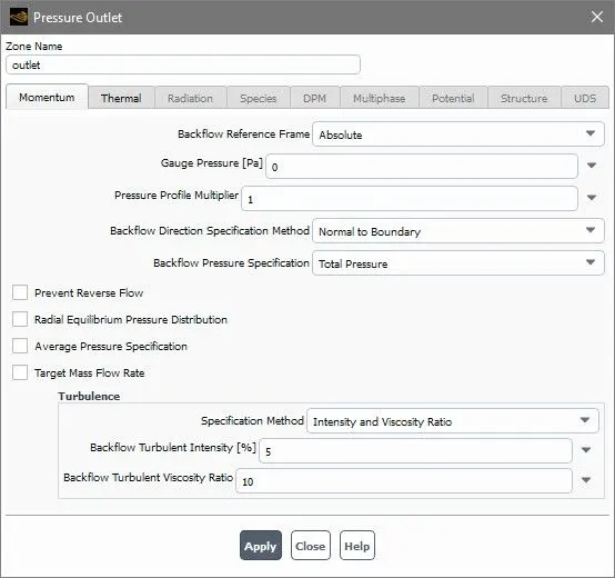
now click on oulet you can see outlet pressure is 0 pa gauge pressure so without any change click apply. here by defult Fluent take oulet pressure equal to one atm. pressure.

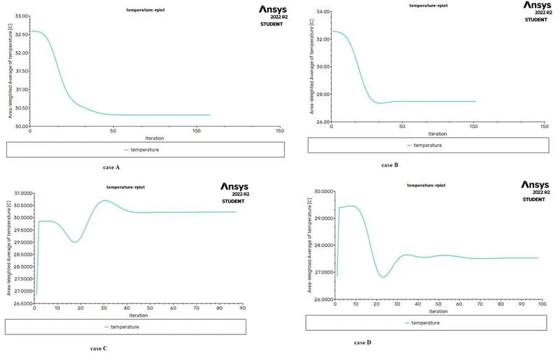
(6) Define the surface plots :- Now click Defination >New >Surface Report > Area-Weighted Average.

Now name temperature and select Temperature as Field Varible and select Outlet surface in create check the Report File and Report Plot and click ok.

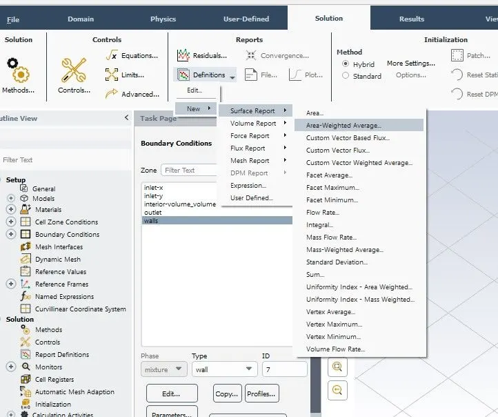
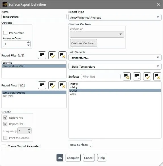
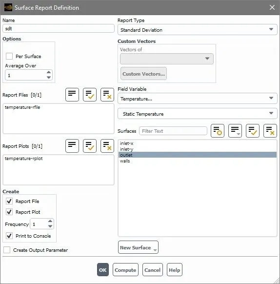
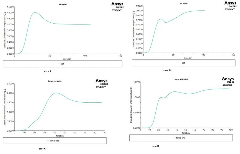
Repete this step for Velocity. and to calculate stander davition of temperature by clicking >New >Surface Report >Standerd devation

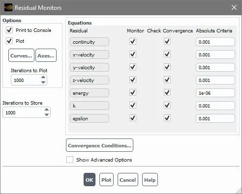
(7) Define convegency :- For this click on Convergency in silution tab or by clicking residual from solution tree.

(8) Solver Run :- Now in solution tab go to Initialization select standard method now click Initialze .

Now go to Run calculation give number of iteration 150 and click calculate to run the solver.

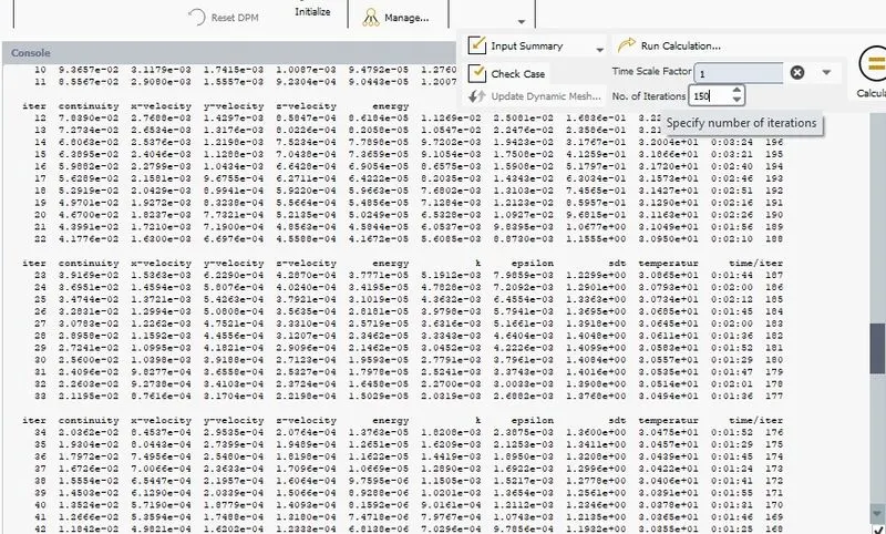
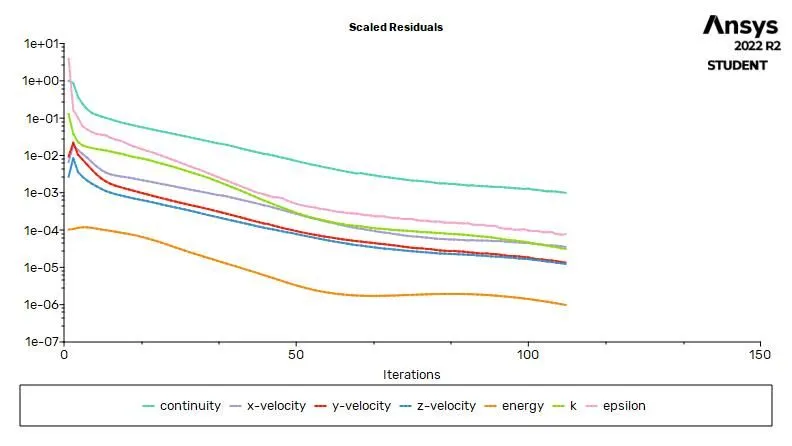
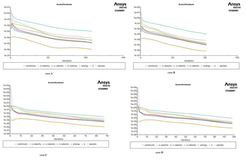
Here on graphic you can see residual drops graps on console can see varibles for each iteration.

if solution is converge the solver is stope ruuning.

(9) Plot Countures

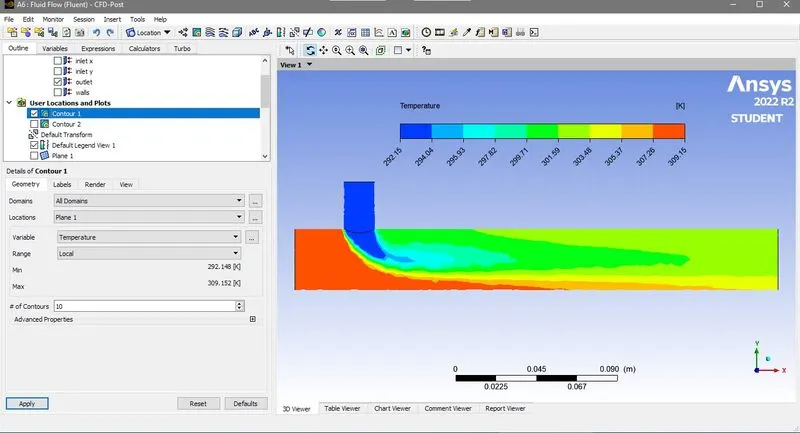
First go to Result Tab creates>palne now click on position drage with mouse and drage palne at center of tee joint and also creates some paralle palne across the length.

Now got to countures > new select filed varible Temperature and select above planes with Inlet-x and Outlet in surface box.

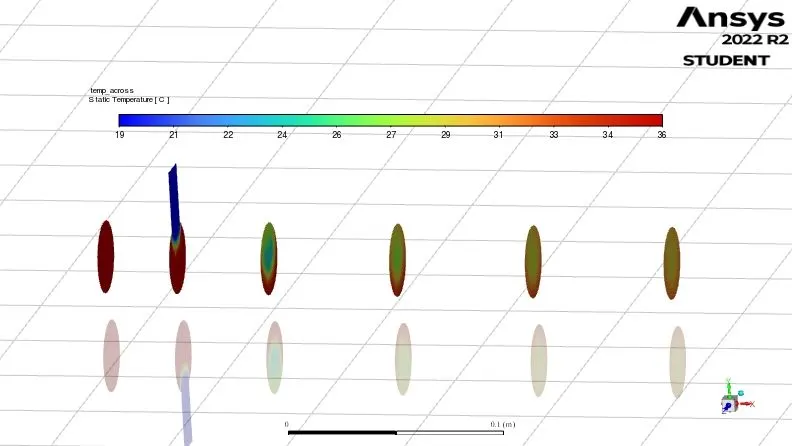
now go to creates>palne> xy plane set z value 0 for center palne. and go to countures > new select filed varible Temperature and select above plane.

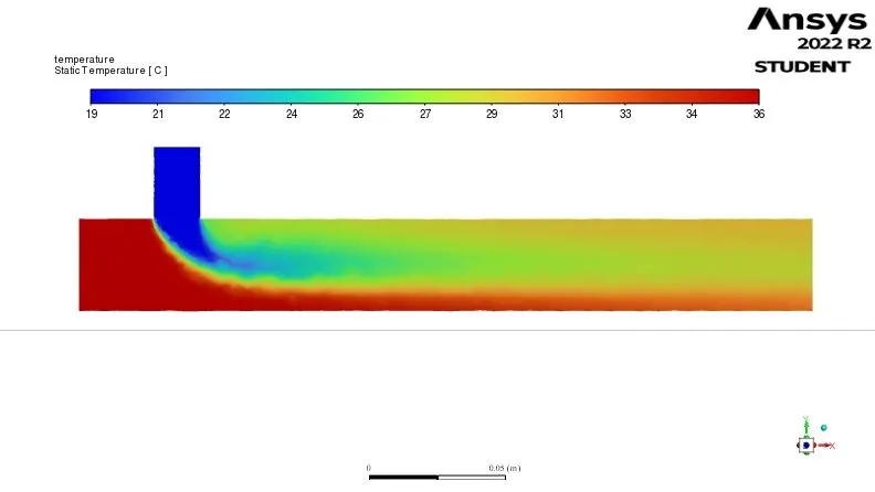
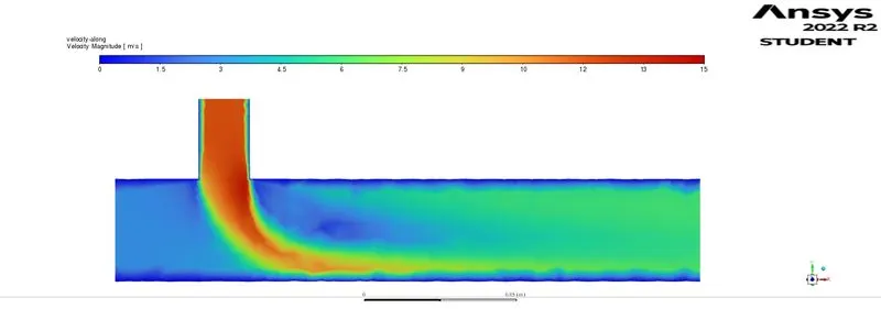
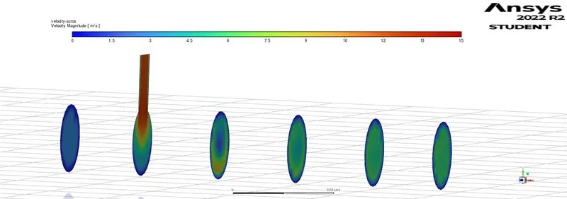
Now by repeting above process we can make countures of velocity also.

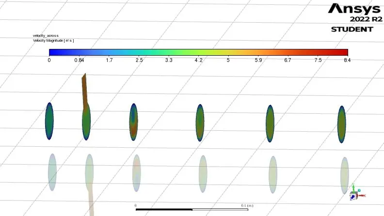
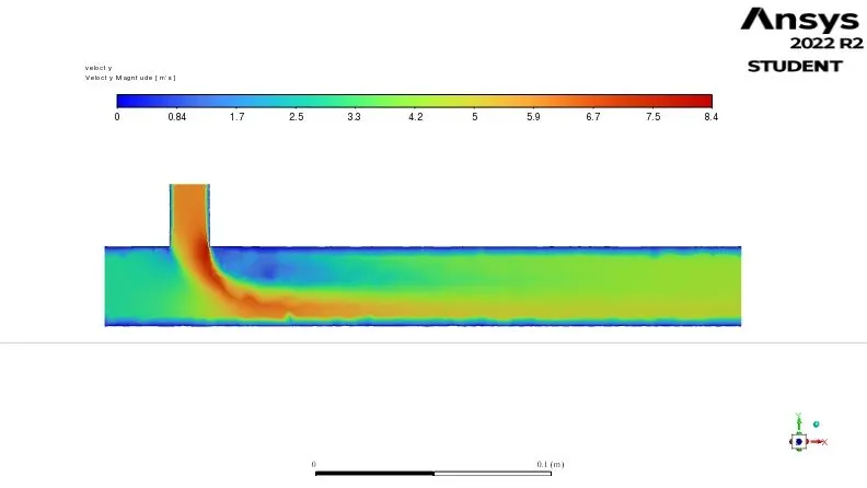
(10) Oulet parameters

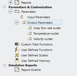
now close the solver enviroment and right click and updates now double click Result to open CFD post

(11) CFD post

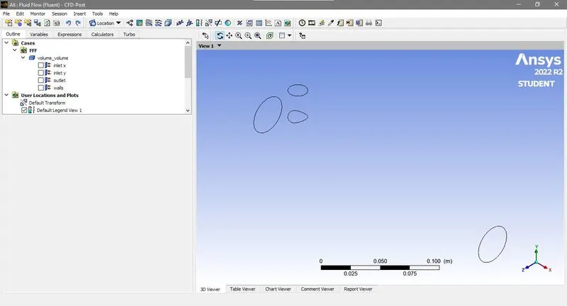
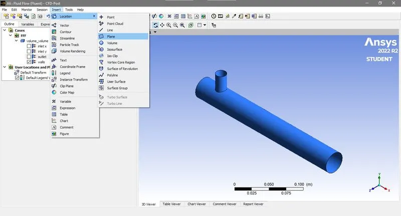
Now select wall faces and change it tranprency

Results

case	mode	cell count	MR	T outlet Analytical	T outlet Numerical	Standard deviation	Number of iterations
A	Long Tee	25601	2	34.11℃	30.307℃	1.0082921	108
B	Long Tee	25601	4	35℃	27.474℃	0.90171764	102
C	Short Tee	22612	2	34.11℃	30.231℃	1.509329	87
D	Short Tee	22612	4	35℃	27.533℃	1.2743509	98

Plots

1. Residual plots

2. Temperature at outlet

3. Standerd devation of Tmperature at outlet

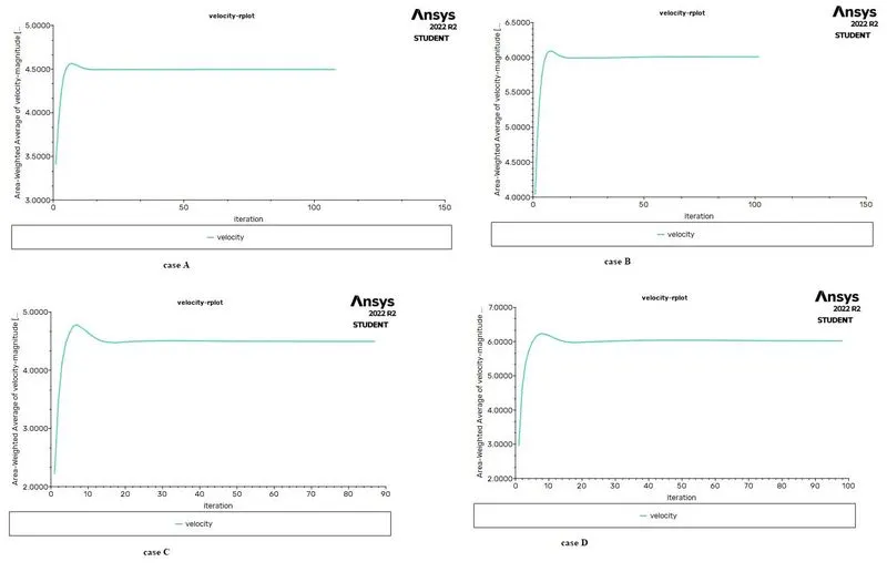
4. Velocity at outlet

Contour plots

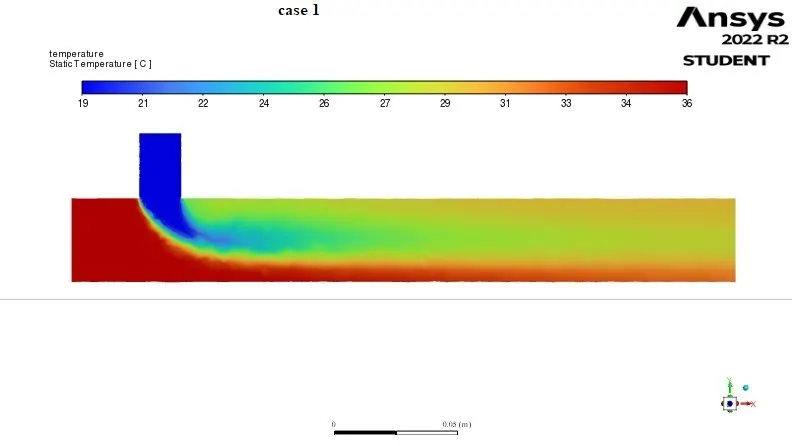
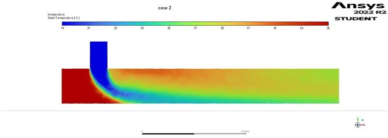
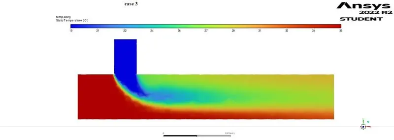
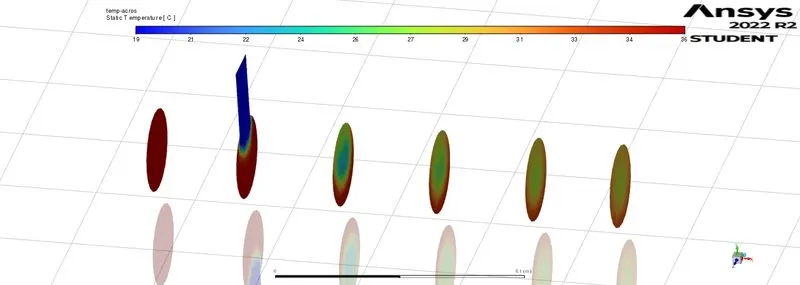
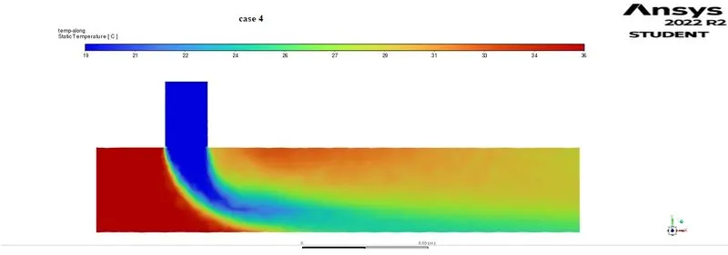
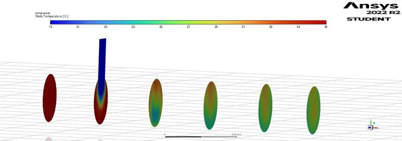
1) Temperature

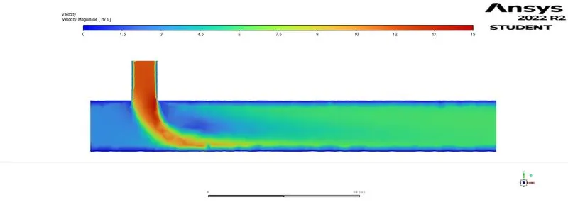
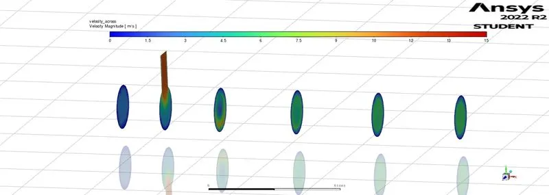
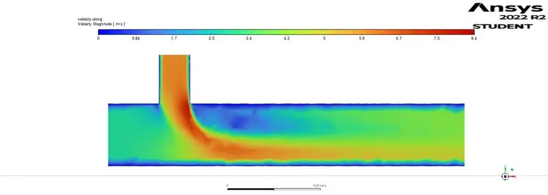
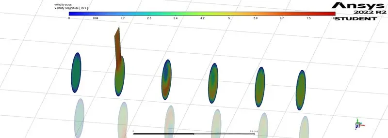
2.) Velocity

Result Summary

1) From the result table long tee model takes more number of iteration as compare to short tee model because of more cell count.
If we compare residual drops plot we can observed in some case residual of continuity equasrion is not achive its convegency value 1e-3 but still the solution is coveged.This is because here output temp. obtain from energy equastion converge the solution
2) From the Temperatue Line plots and result table we can observe Temperature outlet in model having momentum ratio 2 is higher then momentum ratio 4.
This is because as we increase cold inlet velocity result in lesser the flow seperation which you can see in the Temperature counture graph along the length.
As seperation is more in case B and D the mixing efficiency is more then case A and C and you get more less tempereture at outlet .
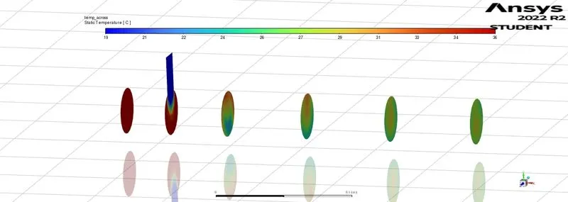
3) Now as we compare standerd devation of temperature at outlet Which is show how much weighted average temperature of oulet deveated from in mean value.
Here shor tee model having more std. devation becuase in short tee model mixture travel length is less so less time is avalable to achive uniform tempereture distribustion accros the length.
we can observed this in Counture plot of temperature across the length.
4) Std. devation of Temperature at outlet is less in cases where momentum ratio is 4. so that as the cold fluid inlet velocity incresess the uniformality of temperature is decrese.

Conclusion

1. To achive better mixing efficiency the model with higher cold inlet velocity is preferred. so that with the momentum ratio efficiency of mixing also increse.
2. To achive better mixing effectiveness we should preferred long mixing Tee model because it have better temperature distribustion at oulet.
3. To achive better mixing effectiveness the model with less cold inlet velocity is preferred. so that with the momentum ratio effectiveness of mixing is decrese.
4. Temperature oulet is inversly perposnal to the momentum ratio in both the model.
5. Error in result of temperture is more in the case where momentum ratio is high.

Downlod the ansys analysis folder of above study from this google drive link

https://drive.google.com/drive/folders/1UZMbijxbb_NJdzMHtdG4-yIptT9AudPt?usp=sharing