Week 5 - Genetic Algorithm

Theory:- The word Optimization is come from latin word 'Optimus' which means 'Best'. Hence is process of getting design point of any function which have multiple parameters. For example while design any aircraft we optimize the lift to minimize drag force for diffrent flight condition. To caluclare these best design point we have to exicuate our process multiple times which take a lot of time so in the matlab there is a globel optimization tool box is use to solve optimization problems.

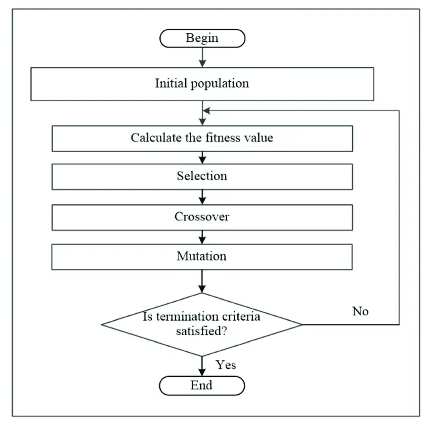
Generic Algorithm is one of the most popular stochastic optimization algorithm often used to solve complex large scale optimization problem in various fields.It is derived from Charles Darwin's theory of evolution, which state that 'It is not the strongest of species that survived ,nor the most integillent , best the one most responsive to change'.

# GA was first introduce by Holland in 1975. It generate high quality solution for both constrained and unconstrained optimazation problem base on natural selection process base on biological evolution.

# It starts with intial set of random solution called population. Each individuals in population is called chromosomes repersenting a solution of the problem at hand.

# The chromosomes evolve through succesive iterations called generation. During each generation, the chromosomes are evaluated using measure of fiteness.

To ceate new generation from chromosomes, called offspring are formed

1. Merging two chromosomes from current generation using crossover

2. Modefing chromosomes using mutation operator

# A new generation formed by

(a) Selecting according to the fitness values sum of parents & offspring

(b) Rejecting others so as to keep the population size that cant filter chromosomes have high probality to select.

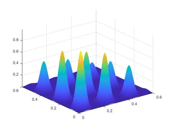
Stalagmite function:- It is a mathematical model which help to generate local minima and maxima. It is three dimentional function is designed in such a way it has lot of local maxima and minima and one global maxima.

The name that arrises from a floor of cave due to accumulation of material deposited on the the floor from celling dripping.

this function is

F(x,y)= (f₁x)*(f₁y)*(f₂x)*(f₂y)

f₁x=(sin(5.1*pi*x+0.5)⁶

f_1y=(sin(5.1*pi*y+0.5)⁶

Here functions f₁x and f₁y are sine power 6 wave minimum value near to 0 and maximum value near to 0.5, so this functions making sufaces of root ant top on xy planes

f₂x=exp(-4*log(2)*((x-0.0667)² /0.64)

f_2y=exp(-4*log(2)*((y-0.0667)² /0.64)

Here functions f₁x and f₁y are exponetional function which makes steep dome surface when it merge with above sine wave function it make mulatiple steep dome curve.

# Matlab function script

function[F] = Stalagmite(input_vector)
x=input_vector(1);
y=input_vector(2);
f1_x=(sin(5.1*pi*x+0.5)).^6;
f1_y=(sin(5.1*pi*y+0.5)).^6;
f2_x=exp(-4*log(2)*((x-0.0667).^2)/0.64);
f2_y=exp(-4*log(2)*((y-0.0667).^2)/0.64);
F=-(f1_x*f1_y*f2_x*f2_y);
end

Here input_vector have two index value which are consider are two input parameter in x and y direction respectivly.

Now function have -ve sine in defination so we can plot using -f then we get desired surface plot as shown bellow.

# Matlab Code for main programe

close all
clear all
clc

% Creating 1D space varibles
x=linspace(0,0.6,150);
y=linspace(0,0.6,150);

% Creating 2D space varibles
[xx yy]=meshgrid(x,y);

% Creating an input vector which contain 2D space data
for i=1:length(xx)
    for j=1:length(yy)
        input_vector(1)=xx(i,j);
        input_vector(2)=yy(i,j);
        % Calling function for each input vector
        F(i,j)= Stalagmite(input_vector);
    end
end

Code explanition

1. In this code first we create two linear space x and y in range 0 to 0.6.Then we create 2D space xx and yy in same range.

In matlab we use linspace to create linear space between 0 and 0.6 we have 150 index. So varible x and y are 150x1 matrix.

In matlab we use meshgrid to create 2D space i.e. two plane xx and yy. were xx & yy are 150x 150 matrix.

2. Now we take a for loop which have an incrment varible i that exicute it on each index of xx plane and inside it an another for loop with increment varible j that exicute it on each index of yy plane. So it is like we are piking up each point of a 3D space. And in this 3D space we create a input_vector of 1x2 dimention.

3. Now we call our function with argument of this input_vectior. As varible input_vectior contain two value in a row.

4. When we matlab complier run Stalagmite function script it cant access main program varible in varible window so here we vlaues of varible input_vector is seprated and store in varible x and y.

5. Now these x and y varible are creating a new varible ' F 'as per defination or formula. Now this varible 'F' is only the varible which step out from function script and x and y are not go out from function so in main program it not replace intial linear varible x and y.

6. Now this output F is one point in 3D space as inner for loop exicute 150 time, then outer for loop only one time so inner for loop again exicute 150 time for each exicution of outer loop. And we get multiple value of varible F which store as a matrix of 150x150.

7. Now we can plot this function F as surfce on 3D space of index xx ,yy and F.

surf(xx,yy,-F)

here we use -F to get peak side because in function we gave it -ve already.

Now the above image is result of this function of space. Now our study is to get maximum point here because we use -F in surface plot other wise we study to get minimum value of surface F and we can also say in both case we study optimum value.

Now we use Genraric Alogritm which is an inbuit function in matlab to get optimum value of F.

The function syntex is

x=ga(fun,nvar,A,b,Aeq,beq,lb,ub,NLC,IC,options)

hear fun is is our Stalagmite function

nvar or nval is number of design varibles.

A is linear inequality coefficient

b is linear inequality coefficient

Aeq is linear equality coefficient

beq is linear equality coefficient

Lb is lower bound

Ub is upper bound

NLC is Nonlinear constrain

IC is Integer constrain

Stopping citeria

ga stops when it reaches the maximum number of generations; by default, this number is 100 times the number of variables. ga also detects if the best fitness value does not change for some time given in seconds (stall time limit), or for some number of generations (maximum stall generations).

There are 3 study of geting GA.

1. Static Behaviour

% Study Of Static Behaviour
num_cases=50;
tic
for i=1:num_cases
    
    [inputs,fopt(i)]=ga(@Stalagmite,2);
    xopt(i)=inputs(1);
    yopt(i)=inputs(2);
end
study1_time=toc

% Ploting
figure(1)
subplot(2,1,1)
hold on
surfc(xx,yy,F)
shading interp
title('Study Of Static Behaviour')
xlabel('X values')
ylabel('Y values')
plot3(xopt,yopt,fopt,'marker','o','markersize',6,'markerfacecolor','r')
subplot(2,1,2)
plot(fopt)
xlabel('Interactions')
ylabel('Function maximum')

Study run time =4.2277

when run program second time it is 4.5043, again run it comes 4.1985. So all time code run time is not same and also result point is also different after two digit in decimal which you can see in below plots.

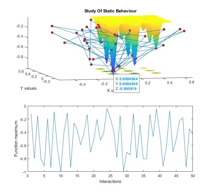
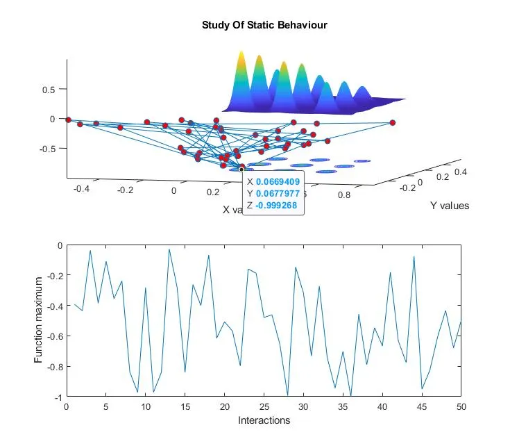
Here above two plot gives result of same study but different is 1st is inverted plot And we use this because the contour of surface projection on xy plane are well visible in it and it stakes less space

2. Stattical behaviour with upper and lower Boundes

% Study Of Statistical Behaviour With Upper And Lower Bounds
tic
for i=1:num_cases;
    [inputs,fopt(i)]=ga(@Stalagmite,2,[],[],[],[],[0;0],[1;1]);
    xopt(i)=inputs(1);
    yopt(i)=inputs(2);
end
study2_time=toc

% Ploting
figure(2)
subplot(2,1,1)
hold on
surfc(xx,yy,F)
shading interp
title('Study Of Statistical Behaviour With Upper And Lower Bounds')
xlabel('X values')
ylabel('Y values')
plot3(xopt,yopt,fopt,'marker','o','markersize',6,'markerfacecolor','r')
subplot(2,1,2)
plot(fopt)
xlabel('Interactions')
ylabel('Function maximum')

Study time 5.7205, 5.6695 qnd 5.8681.

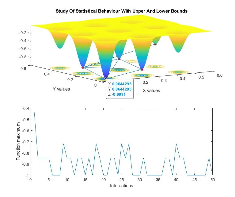
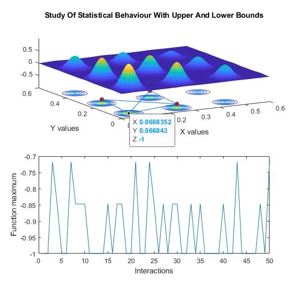
In privous study we do not give any bounds but here we bounds between 0 to 1 so in privous study we get many design point but now we get only those design point which are between the 0 and so 1 so it is reduce to 5 design points.

3. Study of Increasing GA Interactions

% Study Of Increasing GA Interactions
options=optimoptions('ga')
options=optimoptions(options,'populationsize',200);
tic
for i=1:num_cases;
    [inputs,fopt(i)]=ga(@Stalagmite,2,[],[],[],[],[0;0],[0.5;0.5],[],[],options);
    xopt(i)=inputs(1);
    yopt(i)=inputs(2);
end
study3_time=toc

% Ploting
figure(3)
subplot(2,1,1)
hold on
surfc(xx,yy,F)
shading interp
title('Study Of Statistical Behaviour With Upper And Lower Bounds')
xlabel('X values')
ylabel('Y values')
plot3(xopt,yopt,fopt,'marker','o','markersize',6,'markerfacecolor','r')
subplot(2,1,2)
plot(fopt)
xlabel('Interactions')
ylabel('Function maximum')

Here we gave an option for GA i.e. when polulation size comes to 200 stop the interactions.

Here study times are 15.8964, 15.8614 and 15.7343.

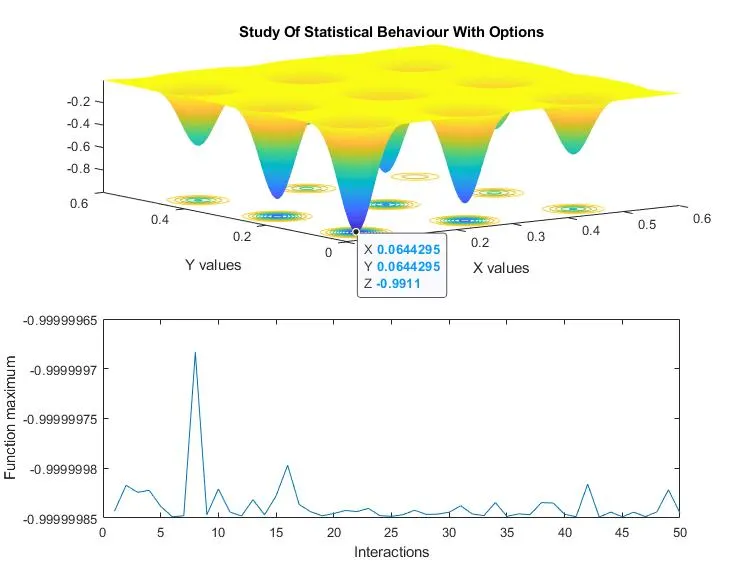
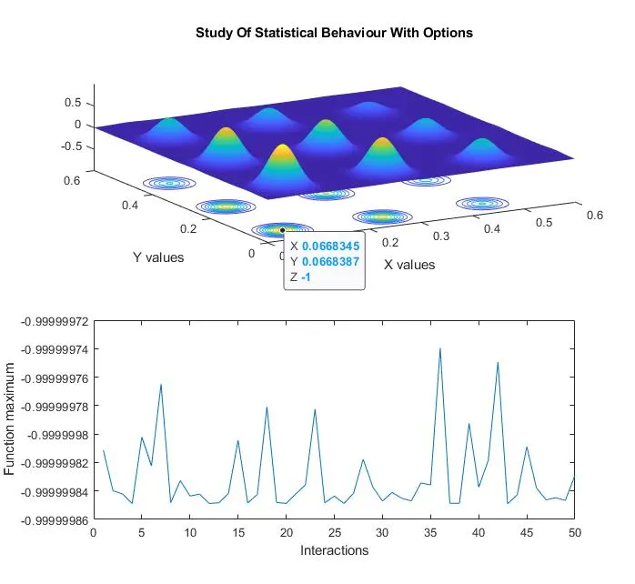
Here we get ony one design point as shwon,

Among all the above study the varition in result is less in study 3 i.e. study with options.

Conclusions:-

1. In this challange we learn Globle otimization and Stalamight function.

2. In this study we learn GA and syntex of ga in matlab and how it work inside the function. The linear and non linear equality and inequality equastions.

3. We also learn use of upper and lower bounds and options in GA.